Chapter 1: The Tropical Rain versus SST Relationship

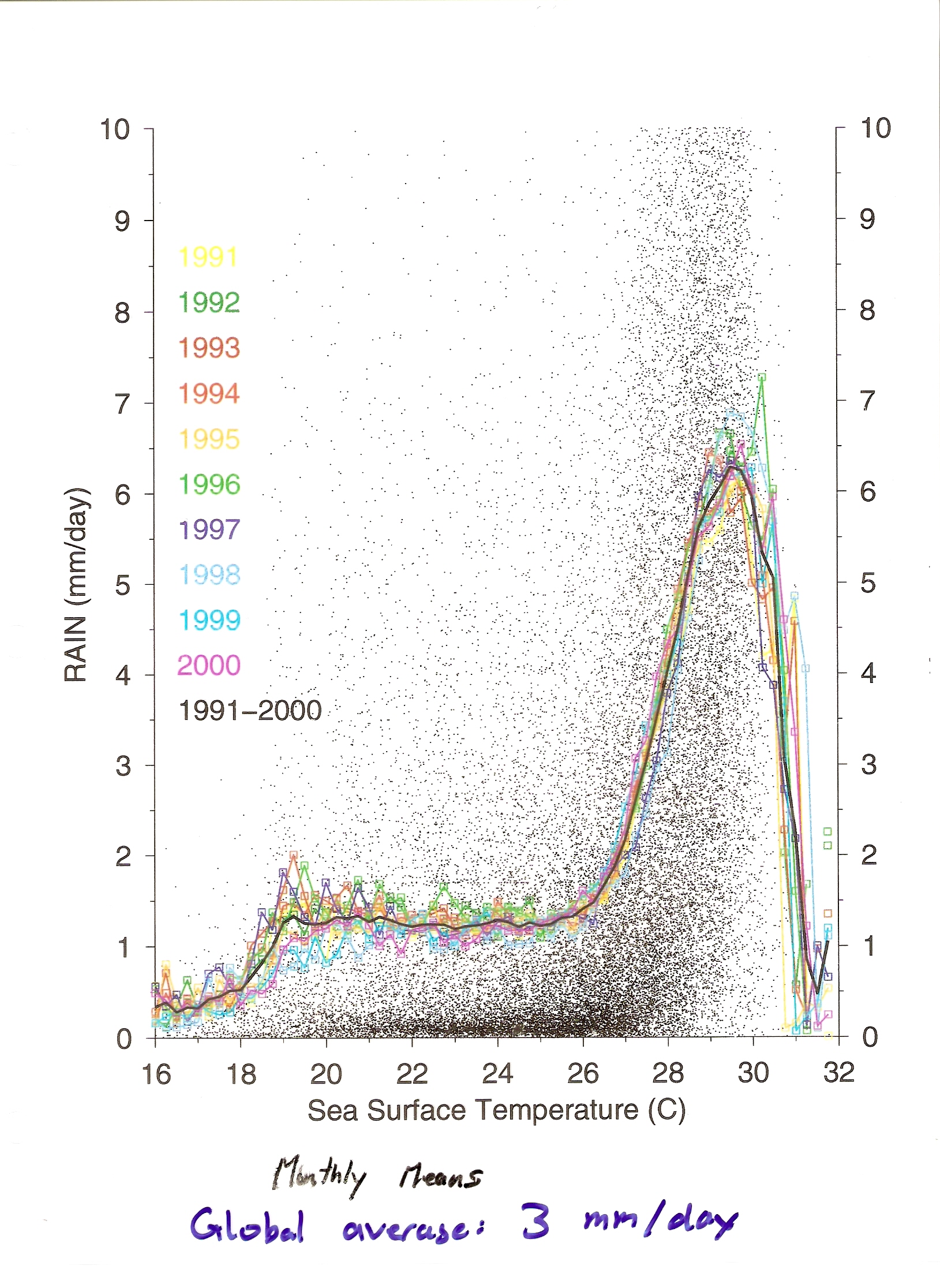
This figure shows the dependence of mean rain rate on SST in the tropics (30 S - 30 N). There are three odd characteristics to this plot. (1) Rain does not increase at all with SST for SST's between 19 C and 26 C. (2) The rainfall rate suddenly increases at a "magic" SST of 26 C. (3) The rainfall rate rapidly decreases as SST's go above 30 C. Why? In general higher sea surface temperatures should be associated with higher fluxes of heat and moisture into the atmosphere, which will favour moist convection (rainfall).

The rainfall decrease at high SST's is usually explained as being due to the fact that in order to generate very high SST's in the tropics, one requires that there be no blockage of solar radiation by clouds for several weeks. Rainfall produces extensive cirrus anvils which reflect solar radiation and cool the underlying ocean. Very high SST's can therefore only occur in their absence, i.e. if very low rain rates persist for several weeks.

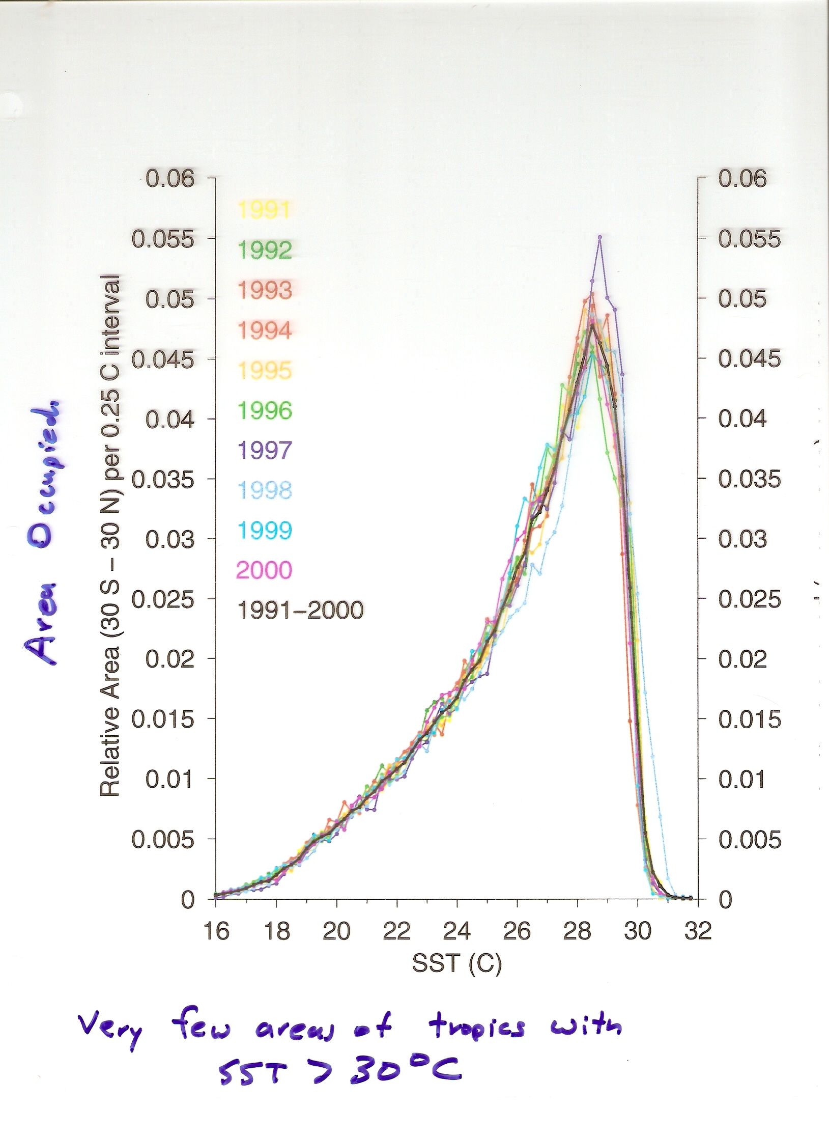
It should be kept in mind that only an extremely small fraction of the tropical oceans have SST's in excess of 30 C, so though interesting, these areas can be a distraction from the basic tendency for higher SST's to be associated with higher rainfall rates. This Figure shows that the most common SST in the tropics is 28 C.

Chapter 1: Three types of precipitation:

(1) Synoptic (2) Convective (3) Orographic

(1) Synoptic Precipitation is produced by low pressure systems. Most winter-time precipitation in mid-latitudes is synoptic precipitation associated with warm and cold fronts. This type of precipitation is produced by "baroclinicity" (horizontal temperature gradients). A highly baroclinic atmosphere has more more gravitational potential energy, which can be used to generate a circulation, and intensify low pressure systems. When the warm air rises up over the cold air in warm fronts, precipitation is generated.

(2) Convective precipitation is produced by some combination of warm, moist air at the surface, and cold air aloft. These conditions favour positive buoyancy of rising air parcels.

(3) Orographic Flow: vertical motion forced by horizontal flow hitting a mountain range generates precipitation on the upwind side of mountain ranges. very important on the western side of North America.

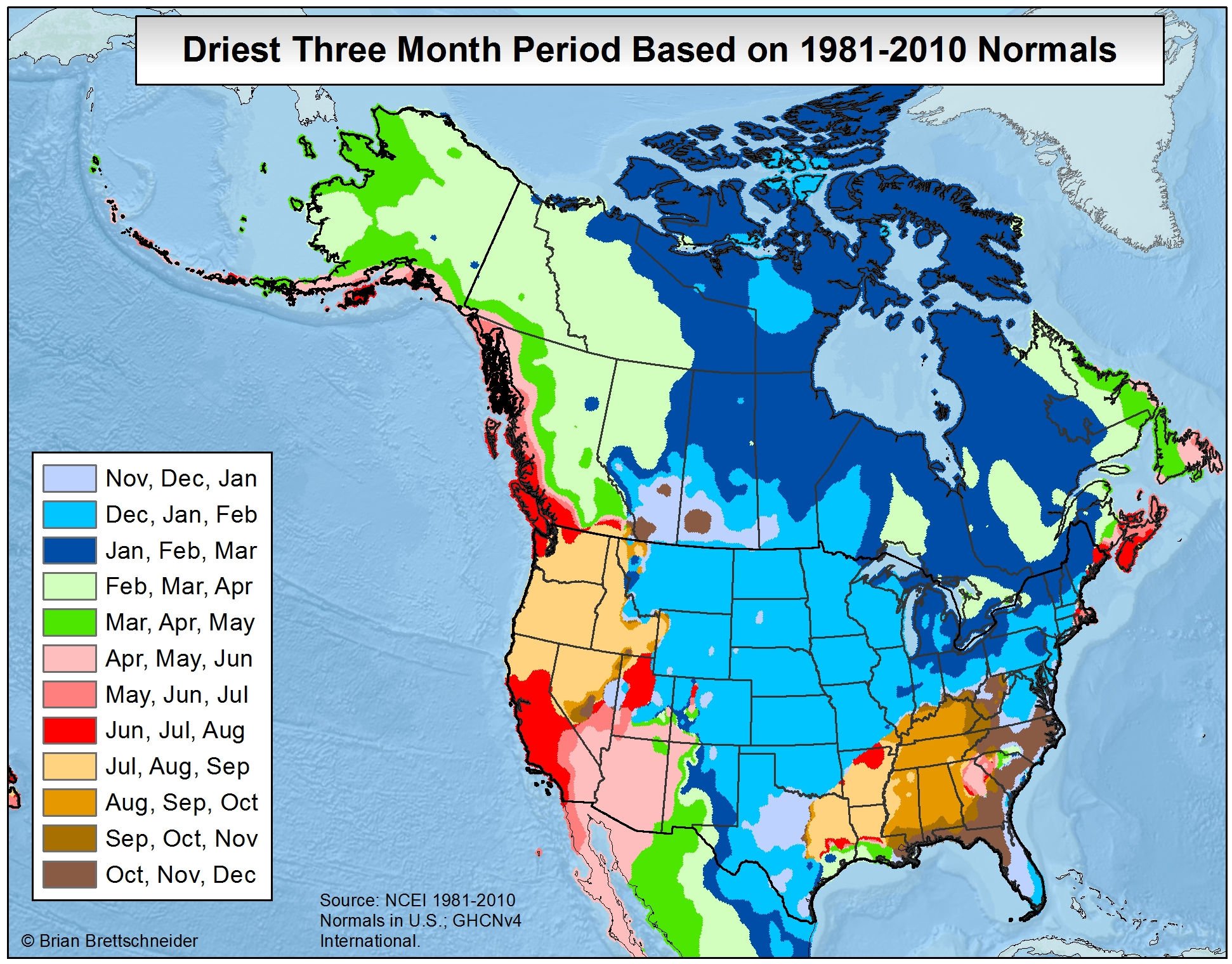
Chapter 1: North American Rainfall

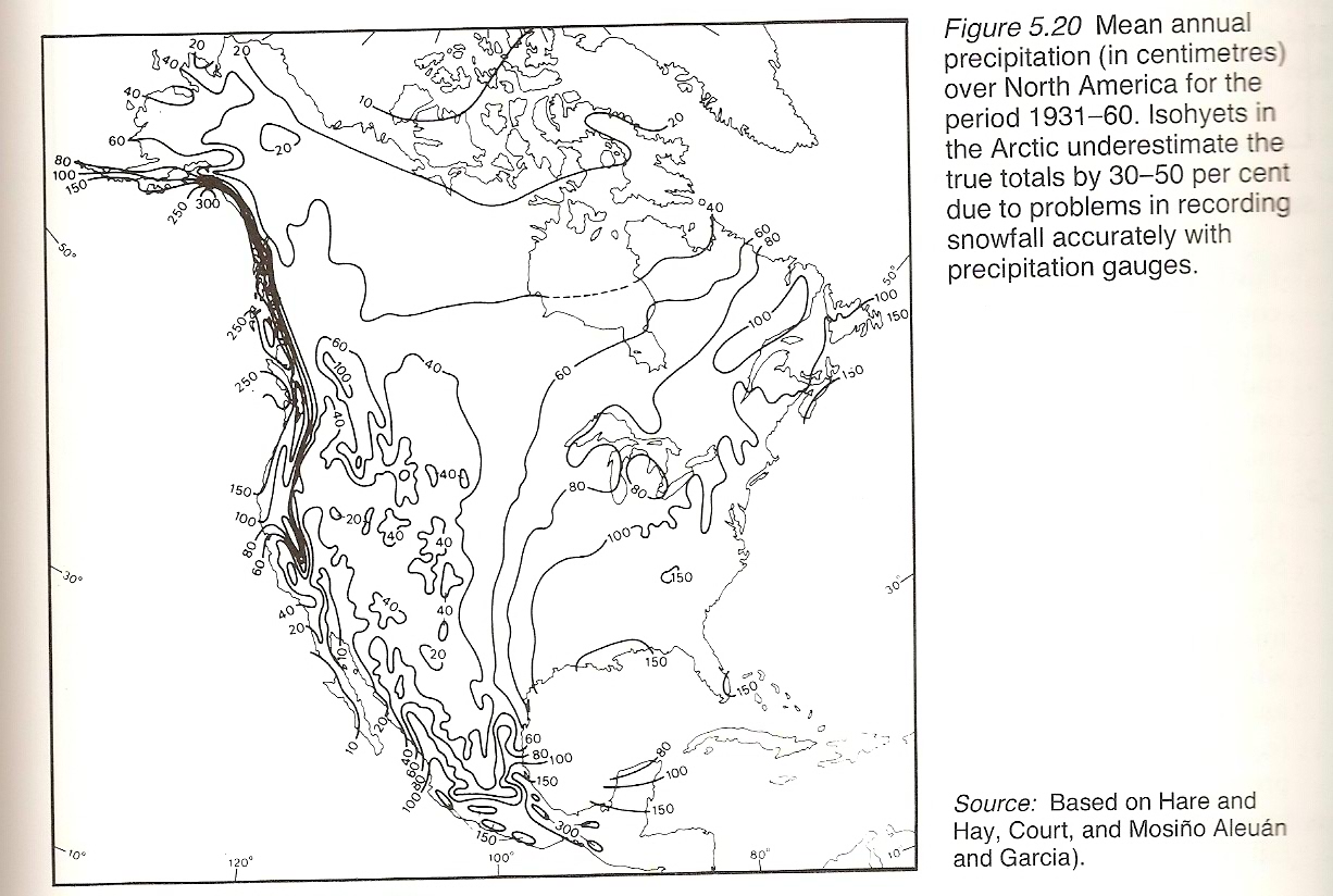
Note that, with the exception of a narrow strip along the Pacific Ocean, Halifax is one of the rainiest places in North America. This is partly due to our proximity to the Gulf Stream. Note also the east-west rain gradient going North - South down the middle of the US, demonstrating the importance of the warm Gulf of Mexico as a source of water vapor for precipitation in the eastern US. Also note that precipitation (in equivalent rain depth) goes to zero as you go further north. This is essentially because the saturated vapor pressure becomes progressively colder with temperature, so that it becomes "too cold too snow" (very much). However, converting snowfall to equivalent rain depth is a sketchy business, partly because the density of snow depends on temperature, partly because wind can make snow gauges inaccurate in collecting snow volume. The strip of high rainfall down the west coast of North America, can be considered orographic rainfall - the forced ascent of moist air from the ocean. It creates dry rain shadows downstream of the mountain ranges.

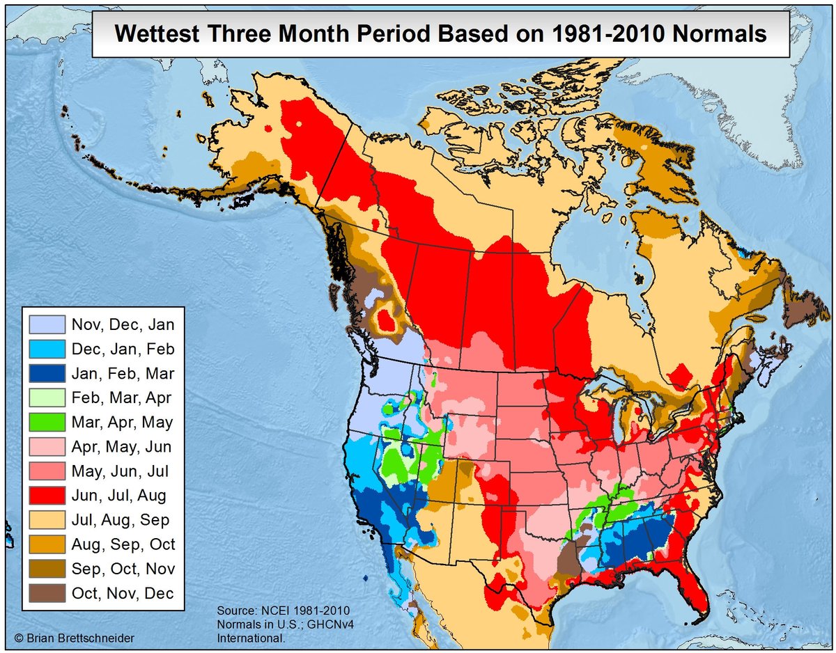
Chapter 1: Seasonal Variation of Northern Hemisphere Rainfall

Chapter 1: Seasonality in various climate regimes

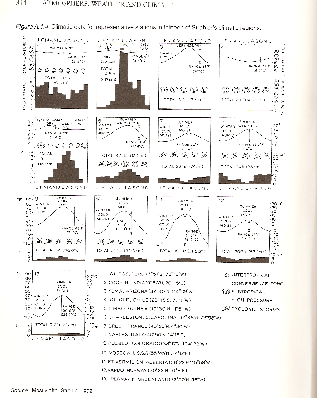
This figure is an attempt to give you a feeling for the different climate regimes which exist on the earth.

Tropical/Monsoonal (India): wet/dry seasons with little temperature seasonality. Monsoon associated with northward movement of ITCZ in NH summer. Monsoon outbreak cools temperatures a little.

Desert Subtropical (Arizona):

Maritime (Norway) : Appreciable rainfall during all seasons due to proximity to ocean. Ocean also reduces temperature seasonality, despite high latitude and huge seasonal variation in TOA SW energy.

Continental (Moscow, Colorado, Alberta): High seasonality in both rainfall and temperature; most precipitation in the summer; no temperature buffering from the oceans; too cold, and too far from a moisture source to have much precip in the winter. However, any snow that does fall tends to accumulate, so snow depths can be significant.

Mediterranean regime (Naples): higher rainfall in winter when the storm track is closer; dry summers since in the subtropical descending zone of the Hadley circulation during this season when the storm tracks have moved into northern Europe.

"Mediterranean" climates would be expected to occur in roughly the 30 N - 40 N latitude band, since 30 N is perhaps the furthest south you might expect winter rainfall to be enhanced by the winter storm track, and 40 N might be the furthest north you might be expect to be influenced by the northward movement of the Hadley circulation in NH summer (and so have reduced rainfall due to having subtropical descent). However, there are many places in this latitude band that do not have a Mediterranean climate. For example, the southeast US and Florida have significant rainfall in the summer, (and some of the strongest convective storms on earth) despite being at that time of the year "subtropical". Nice, (in southern France) is at 45 N, and perhaps even Victoria BC (50 N), could be considered to have Mediterranean climates (hot drier summers, cool moist winters). The dry summers are not so much due to being in the descending zone of the Hadley circulation, but downstream of a high at this time of year (Pacific and Bermuda high respectively).

The climate at any location is determined by a multiple of factors in addition to latitude: proximity to the ocean, temperature of the ocean, altitude, the existence of nearby mountain ranges, and its location relative to nearby climatological highs and lows. For example, the lack of summer rainfall in Nice would be partially due to it being influenced by subsidence (sinking) from the Bermuda High. This sinking aloft would heat the atmosphere, and tend to suppress the development of convective storms. Similarly, being downstream of the Pacific High in summer would reduce the summer rainfall of Victoria, and make it effectively "subtropical" at this time of year (of course the Pacific Ocean prevents Victoria from having the classic hot Mediterranean summer). Rainfall in the southeast US is strongly affected by the heat low that develops over the interior of North America during summer. This heat low, in combination with the Bermuda high, helps transport warm moist air from the Gulf of Mexico northward and moistens the eastern half of North America. Italy is a long narrow peninsula with quite high mountains, surrounded by warm Mediterranean waters: you might think that these factors would favor the development of a convergent sea breeze circulation and orographic thunderstorms over Italy in summer, and increase summer rainfall in Italy. Apparently, this tendency is sufficiently offset by subtropical and Bermuda high subsidence, which would again tend to suppress the development of thunderstorms, so that it doesn't increase summer rainfall by very much. However, Florida has a very strong convergent sea breeze circulation in summer which gives rise to afternoon thunderstorms almost every day.

Supplemental Material for Chapter 2

There are 110 figures here. Most relevant to this class are : 7, 8, 10, 12, 15, 20, 22, 31, 33, 37, 40, 42, 49, 55, 58, 59, 60, 61 (Three carbon cycles: important), 65, 67, 73, 81 (snowball earth), 82, 88, 91, 92, 95, 97.

Chapter 2: Gyre circulations in the Southern Hemisphere?

Figure 2.4 shows that gyre circulations do exist in the Southern Hemisphere Ocean basins, just as in the Northern Hemisphere, but are weaker. These circulations help transport tropical heat toward the Southern Pole, just as in the Northern Hemisphere. However, the Southern Hemisphere has a current called the Antarctic Circumpolar Current which is a westerly (or eastward) current going around Antarctica. Such a current does not exist in the Northern Hemisphere, because it would be blocked by the Asian and North American continents. In the Southern Hemisphere, the Drake passage between South America and Antarctic allows this circumpolar current to exist.

Chapter 2: Thermohaline Shutdown?

You may have heard about the possibility of a cooling in Europe due to a weakening of the thermohaline circulation. It is likely that this fear is overstated. In the current climate, deep water formation occurs in the North Atlantic because the effect of cold atmospheric temperatures (and brine rejection) in increasing the density of seawater is stronger than the freshening (lightening) effect due to the local excess of precipitation over evaporation. In mid-latitudes and polar regions, some of the precipitation originates as evaporation from the subtropics, giving rise to a net poleward transport of water vapor in the atmosphere. If, due to global warming, the temperature difference between the tropics and polar regions were to decrease (likely), or the Arctic freshening effect were to increase due to increased precipitation, or there was a large release of ice and/or fresh water into the North Atlantic from a rapid collapse of the Greenland ice sheet, it is reasonable to think that the thermohaline circulation would slow down.

A decrease in the thermohaline circulation is possible. However, our understanding of the thermohaline circulation is still quite primitive. The mechanisms that drive the downward transport of water at high latitudes are well understood. But the mechanisms whereby water parcels rise upward toward in the tropics and elsewhere (thus completing the circulation) are controversial. If we do not have a complete understanding of a circulation, it is not clear that we can predict its evolution.

It is also not clear that a decrease in the thermohaline circulation would have much effect on the climate of Europe in the short term. Victoria BC (50 N) has a climate comparable to that of England in the winter. In both cases, it is mainly due to being downwind of a huge reservoir of heat (Pacific and Atlantic Oceans respectively). Oceans absorb the warmth of the sun during the summer months and release this stored heat during the winter. There is no deep water formation in the Pacific, and no thermohaline circulation: only the wind driven gyre circulation. The clockwise North Atlantic and North Pacific gyre circulations help transport heat to the North Atlantic and North Pacific, and will continue as long as we have surface westerlies, and easterly trade winds, i.e. as long as the earth continues to rotate.

Although a European cooling due to a shutdown of the thermohaline circulation as unlikely, we should still care about its future evolution. The overturning thermohaline circulation plays an important role in gas exchange (absorbing much of our CO2 emissions), the transport of heat to the deep ocean interior (thus slowing down global warming), and the existence of nutrient rich upwelling regions in the oceans (e.g. the Galapagos).

Much of the interest in the role of a possible change in the thermohaline circulation in cooling Europe originates from paleoclimate evidence that large impulses of fresh water from the North American ice sheet did have a large cooling effect on Europe. This happened about 12,000 years ago and is called the Younger Dryas (see Figure 2.35). It is important to keep in mind, however, that the North American ice sheet was larger than the current Antarctic ice sheet, which is 10 times larger than the Greenland ice sheet. It is also likely that a huge ice or land dam created a huge inland lake in North America, and that this lake then drained into the North Atlantic very quickly. It is not clear that even a rapid Greenland melt would give rise to a large enough fresh water pulse to cool and freshen the North Atlantic in such a way as to regionally cool Europe enough to counteract the overall global warming trend. And if the thermohaline circulation did shut down, it would presumably decrease the oceanic drawdown of CO2 from the atmosphere, potentially increasing the upward trend of CO2 in the atmosphere.

Chapter 2: Thermohaline Reversal?

In the above paragraph, I suggested that a widespread cooling of Europe due to a thermohaline shutdown shutdown (due to the current increase in CO2 concentrations in the atmosphere) was unlikely. However, there is paleoclimate evidence that the overturning circulation in the ocean may have been quite different in the past than at present, and it is likely that the thermohaline circulation will evolve in response to global warming. It is quite conceivable for deep water formation to occur in the subtropics where seawater at the surface is most saline. This warm salty water would then presumably come back to the surface in the poles where freshening occurs. Evidence from isotopes suggests that ocean bottom temperatures in the North Atlantic were near 15C in the past (100 million years ago), and a reversal of the thermohaline circulation is a candidate explanation for these high temperatures. This would also help explain the existence of tropical plants and animals in the Canadian high Arctic at this time. The ocean may have effectively provided a short circuit for warm tropical water to emerge in the Arctic without being cooled by the atmosphere along the way. This is one solution to the "equable climate problem" (warm to moderate temperatures on the whole earth). It seems difficult for climate models to generate these types of climates (reduced equator to pole temperature gradients), without invoking some change in ocean circulation. By itself, the atmosphere does not seem able to transport tropical heat to the poles sufficiently rapidly.

Chapter 2: Lifetime of the Thermohaline Circulation

It takes on the order of several thousand years for a water parcel to complete one loop of the thermohaline circulation (obviously its identity is to some extent smoothed out along the way by mixing). This has implications for the rate of global warming due to increased CO2. Water parcels are continuously coming into contact with the atmosphere (as they reach the surface) whose last contact with the atmosphere would have been several thousand years ago. This water must now come into balance with the current slightly warmer atmosphere (on average). The slowness of the thermohaline circulation, coupled with the huge heat capacity of the ocean, therefore exerts a tremendous drag on the rate of global warming. The ice sheets are another important drag on the rate of global warming due to increased CO2.

Chapter 2: Why no Deep Water Formation in the North Pacific?

The reason appears to be that salinity is higher in the Atlantic Ocean than the Pacific Ocean, so that water in the Pacific is less dense and can't sink (i.e. can't break through the higher density layers beneath it). The salinity difference may have its origin in the transport of water vapor from the Caribbean to the Pacific Ocean across the isthmus of Panama, due to the trade winds. This transport would freshen the Pacific. More generally, there is usually an excess of precipitation over evaporation over land masses, as suggested by the existence of rivers. The Atlantic Ocean is smaller and would therefore tend to be a relatively greater exporter of water vapor to its adjacent continents. To the extent that this export was not balanced by river input, it would make the Atlantic Ocean more saline.

Chapter 2: Inferring Circulations from Tracers

A conservative tracer is a property of an air or water parcel that is constant, or nearly constant, as the parcel moves through whatever medium it is in. Commonly used dynamical tracers in the atmosphere are potential temperature, potential vorticity, and moist static energy. There are also chemical tracers such as ozone, specific humidity, carbon dioxide. Of course, no tracer is perfectly conserved, so it is necessary to use a tracer with a lifetime appropriate to the dynamical problem you are interested in learning about.

One of the first examples of a tracer being used to infer the existence of a circulation was the use, during World War 2, of specific humidity measurements in the lower stratosphere over England to infer the existence of the Brewer Dobson circulation, and more specifically that air entered the stratosphere by crossing the tropical tropopause (and being "freeze-dried" in doing so). Water vapor is a useful tracer for this problem because there are few clouds or precipitation processes in the stratosphere that could change the specific humidity of an air parcel, and also because the tropical tropopause imposes a very specific and unique boundary condition on the stratospheric entry water vapor mixing ratio (about 3 parts per million, lower than found anywhere else). Note that the specific humidity is a much less useful tracer in the troposphere, due to cloud processes and surface evaporation. The water vapor mixing ratio of an air parcel in the stratosphere does in fact increase due to the oxidation of methane (CH4), but this would not have been known at the time, and in any case is quite slow. Temperature and relative humidity are not tracers in the atmosphere. This is because of the compressibility of the atmosphere: an air parcel that rises to a lower pressure will expand, become colder, and will have a reduced saturated water vapor pressure (hence relative humidity goes up).

Temperature and salinity have been used in the ocean to infer the existence of some aspects of the thermohaline circulation. There are no internal heat or salt sources in the ocean (dissipative heating is weak and thermal and salt diffusion and mixing slow), so that the temperature and salinity of a water parcel can only be significantly changed via contact with the atmosphere. The (T,s) signature of a water parcel can therefore be considered an atmospheric imprint on a water parcel, that provides it with a memory of its origin, since certain (T,s) values are more characteristic of particular ocean surface regions than others (e.g. see discussion on why the Atlantic is saltier than the Pacific).

The use of this type of inductive reasoning based on tracers is more common in geophysics than the physical sciences, and is a nice complement to the more deductive mechanistic type reasoning based on the application of the governing dynamical equations. We learn about circulations by seeking a convergence between the two types of arguments.

Chapter 2: Cryosphere

Chapter 2: Figure 2.34 - Summer NH insolation and rapid

decreases in Ice Volume

This figure is a bit confusing because the time axis is so compressed. The upper ice volume curve shows the sawtooth pattern characteristic of slow ice accumulation followed by rapid melt. The lower plot shows a blue curve togethor with a red curve. The lower red curve shows the amount of insolation (sunlight) during the summer in the Northern Hemisphere. The rapid melts of the upper blue curve occur when large ice volumes are strongly out of balance with the orbital forcing. The peaks in the lower red curve (hot summers) then drive rapid decreases in the upper ice volume curve.

Why are changes in ice volume mainly determined by summer sunlight in the Northern Hemisphere? Changes in the volume of the Antarctic Ice Sheet do not appear to be as responsive to changes in temperature as the ice sheets in the Norther Hemisphere. The area if the Antarctic ice sheet can't increase that much because it is constrained by the ocean. The Antarctic ice sheet probably can't get much higher because its top would get even colder and dryer, thus further reducing snow accumulation. The ice sheet probably does not shrink too much in response to a warmer climate, at least initially, because an increase in temperature would increase snow accumulation (because much of the surface of the ice sheet is now so cold and dry.) Of course, the jury is still out, but a significant change in the volume of the Greenland ice sheet over the next 50 - 100 years is more likely than a significant change in the volume of the Antarctic ice sheet.

Chapter 2: Should we be worried about the next Ice Age?

We are currently living in an interglacial. For the past several million years, there has been a warm period, or interglacial, about every 100,000 years which lasts about 10,000 years. The current interglacial is called the Holocene. During the roughly 90,000 year cold periods, the glaciers periodically advance and retreat. Although the current interglacial would ordinarily likely end within the next few thousand years, it takes several tens of thousands of years for the ice sheets to build up, and the maximum cooling to be achieved. The warming that will likely occur over the next few hundred years from the buildup of greenhouse gases is likely to delay the next ice age. Global averaged temperature during ice ages are about 4 C cooler than during interglacials. Given that it takes about 50,000 years to produce this cooling, the cooling rate is roughly 0.01 C/century. The warming rate due to enhanced CO2 is likely to be in the range 2 - 4 C/century, or several hundred times faster than the ice age cooling. In the timeframe of the next several hundred years, temperature changes associated with changes in orbital forcing are not likely to be relevant.

Chapter 2: Greenland Meltwater Ponds

The surface of the Greenland Ice Sheet is in some places quite hilly with complex topography of lakes and streams. Here is a picture:

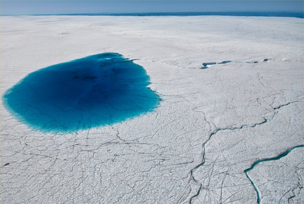
Meltwater lake and streams on the Greenland Ice Sheet near 68 N at 1000 meters altitude. Photo by Ian Joughin.

Chapter 2: Negative Trend in September Arctic Sea Ice

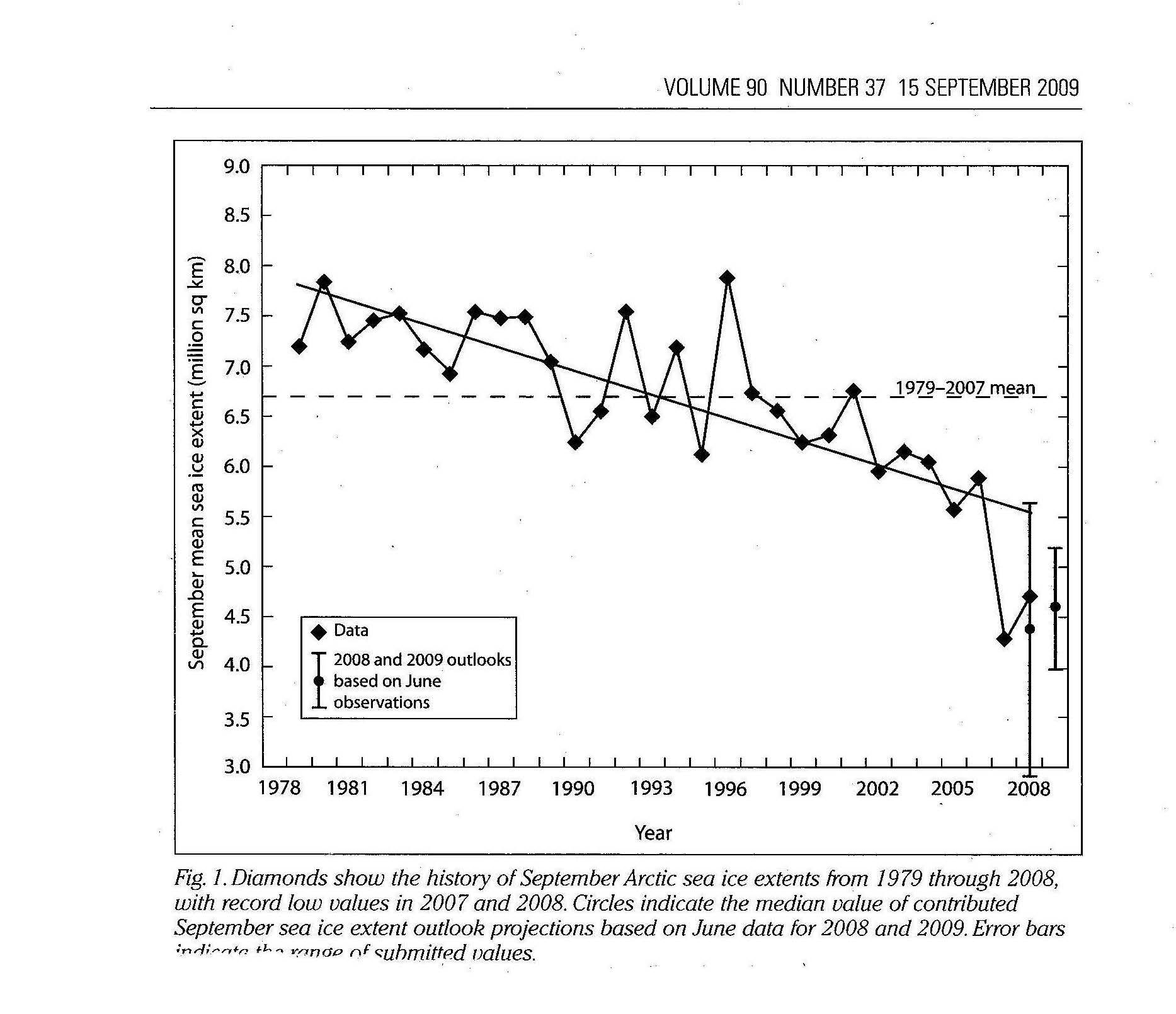
September Arctic sea ice is now likely down to about half of what we had in the mid 1970's. It is hard to go back further in time due to a lack of satellite measurements. There is also a downward trend in March sea ice area, but it is much weaker.

Chapter 2: Handout - Climate of the Last 100 Million Years

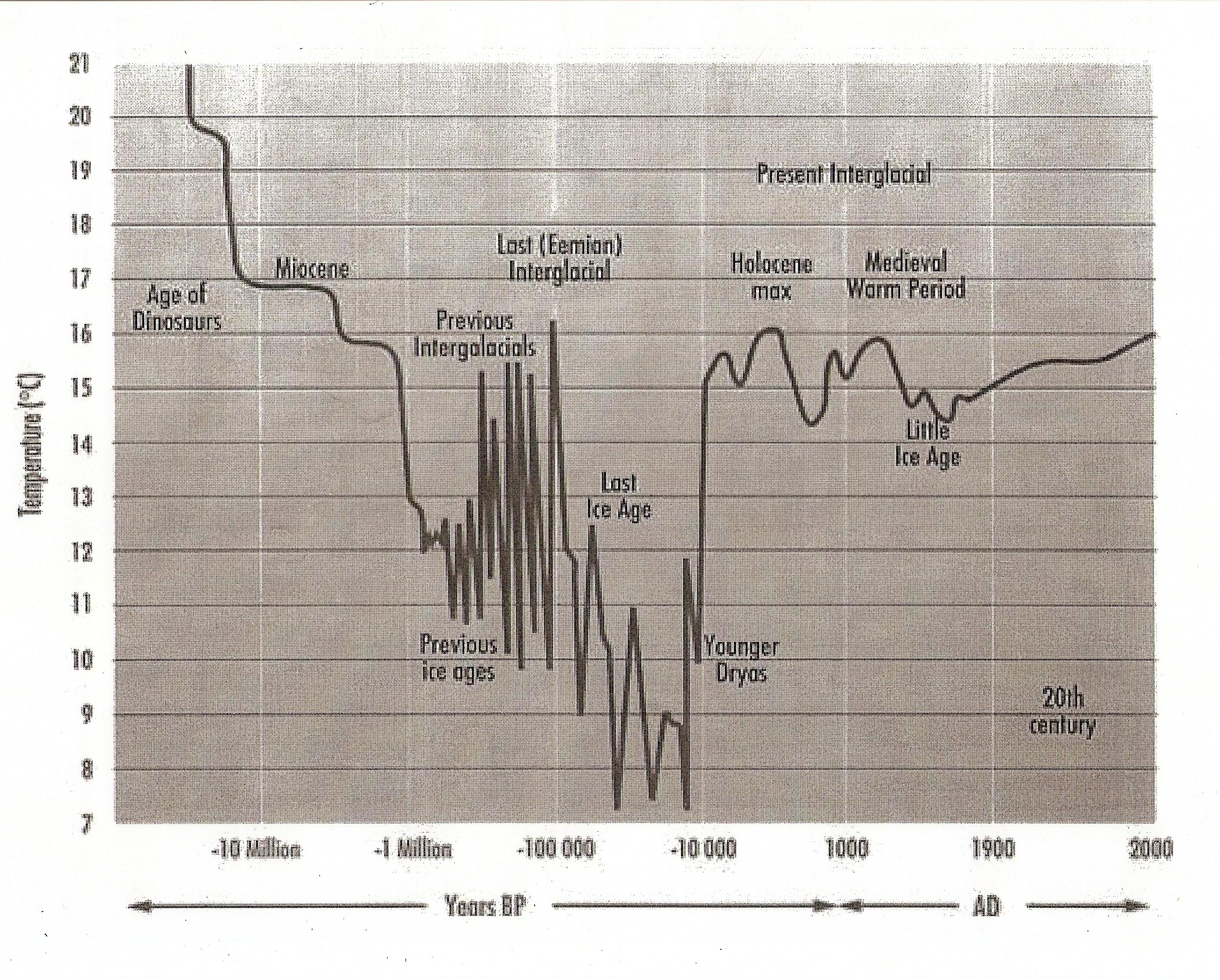
This figure is a summary of the climate of the last 100 million years. A logarithmic scale has been used on the time axis to be able to show slow long climate changes together with more recent faster climate changes.

The temperature versus time plot shows a lot of information: a long timescale "tectonic" cooling associated with decreasing levels of CO2 in the atmosphere starting 100 million years ago, the onset of an ice volume response to orbital forcings (i.e. glacial/interglacial cycles) 1 million years ago, the Younger Dryas cooling as we came out of the last ice age probably caused by a huge release of freshwater into the North Atlantic, and the more recent Holocene (interglacial) warmth. A true appreciation for climate change requires knowledge of biochemistry, plate tectonics, ocean circulation, ice sheet dynamics, and atmospheric climate feedbacks.

It is important to place the current climate debate into a longer term climate context. In my experience, there are two types of lessons people draw in the face of this almost bewildering climate complexity. Many geologists are very familiar with the evidence for climate change from the geological record, and are therefore aware of the difficulties in distinguishing current climate trends from natural variability. This sometimes leads them to adopt the position of a ''climate skeptic'', someone who is reluctant to attribute current climate change to human induced changes in CO2. They believe there is sufficient noise in the climate system that the attribution question becomes unanswerable, or that the "human induced" climate noise must be smaller than the "natural" climate noise.

On the other hand, one could be equally impressed by the degree to which huge climate changes in the past have been apparently induced by relatively modest changes in radiative forcing (mainly from CO2 and orbital changes), and that this suggests that the climate sensitivity of the earth is quite large, i.e. that positive climate feedbacks (water vapor, ice albedo, clouds, CO2) dominate over possible negative feedbacks that might stabilize the earth's climate. For example, we do not yet have a full understanding of ice ages. However, if one believes that there is some negative feedback in operation that will negate any future warming associated with CO2 increases, then it becomes much more difficult to explain the sensitivity of the earth's climate to orbital forcings, and therefore, the existence of ice ages. If it existed, such a stabilizing mechanism would have also moderated the temperature variability during the ice ages in the past. Apparently, it has not.

Chapter 2: CO2 and Heating from Radioactive Decay

The interior of the earth is heated by radioactive decay. This is the heat source which drives plate tectonics. In the absence of plate tectonics, carbon would accumulate in the earth, and the atmospheric concentration of CO2 would become smaller and smaller. The volcanic source of CO2 would shut down. So, even though the internal source of heat to the earth is tiny compared with heating from the sun, it is magnified due to its role in the carbon cycle, and is essential to life on earth.

The volcanic outgassing of CO2, and the geological removal of CO2 from the atmosphere due to carbon burial (formation of coal, limestone, etc.) do not have to balance at any given time. During periods of increased volcanic activity, CO2 should go up. During periods of increased mountain building, CO2 should go down. For the past 100 million years, it appears as if mountain building in the Himalayas (exposure of new rock to the atmosphere and increased weathering and carbon burial) have decreased CO2.

Chapter 2: Snowball Earth

In the past, it appears that CO2 concentrations have at times gotten so low that the earth has been almost completely covered with ice - the so called snowball earth - such that almost all life became extinct. How do you get out of the snowball? Rock weathering shuts down as rain/snow stop, so CO2 stops being removed from the atmosphere. There is no reason for volcanism to stop, however, so that the CO2 level of the atmosphere should eventually go up due to volcanic outgassing of CO2 through the ice. Eventually, atmospheric CO2 is high enough that it melts the ice very quickly. The resulting formation of oceans would increase the level of water vapor in the atmosphere. Since water vapor is an extremely strong greenhouse gas, the snowball earth may potentially be followed in quick succession by a very warm earth.

Chapter 2: Circulations: Forcing, Timescales, and Dissipation

The most basic questions to ask about any circulation are: (i) What drives the circulation (creates kinetic energy)?, (ii) what is its timescale?, and (iii) how is its kinetic energy dissipated? If I sit in a bathtub and use my hands to drive a rotation around the tub, this is considered a "mechanically forced" circulation. The tides would also be considered to be mechanically forced circulations, driven by the gravitational attraction of the sun + moon, and the North Atlantic gyre is a circulation mechanically forced by the atmospheric wind. The timescale of the bathtub circulation would be the time it takes a water parcel to execute one loop, perhaps one minute. The kinetic energy energy would be destroyed by friction with the sides of the bathtub. The "spin down" time of a circulation would be the time it would take the kinetic energy of the circulation to go down by half once the mechanical forcing is removed. The spin down time can be much larger or much smaller than the timescale of the circulation itself.

We have discussed the following circulations: Brewer Dobson, Hadley, thermohaline, North Atlantic gyre, and mantle convection. You should be familiar with what drives each of these and the approximate timescale of each.

Chapter 2: The three carbon cycles - figure 61

I don't think the text explicitly discusses the carbon cycle in terms of three distinct cycles, but I think it is helpful to make these distinctions.

(1) Short term organic carbon cycle: includes the seasonal growth of leaves/grass in the spring + decay in the fall (timescale ~ 6 months), growth and decay of trees (timescale up to thousands of years), growth and decay of plant/animal biomass in the ocean, both in the surface waters and at the bottom, etc. The main point here is that the organic carbon in the plant biomass is directly converted back to CO2, rather than being converted to some longer term geological sink, as in cycles 2 and 3. Peat (think of bogs) is difficult to categorize. If it burns, as it would tend to during dry conditions, peat would be participating in the short term carbon cycle. However, peat is also a precursor to coal, which would be considered a long term geological sink of carbon. In this case, the peat would be participating in cycle 2.

(2) Long Term organic: geological burial of carbon in the form of coal, oil, gas, etc. Most oil tends to form at the bottom of the ocean under anoxic conditions. Only a tiny fraction of plant biomass is lost via long term organic geological burial. However, once there, Table 2.3 shows that it has a residence time of 200 million years, so has accumulated to 20,000 kg/m2 (or about twice the mass density of the atmosphere). We are currently in the process of extracting and burning the economically recoverable part of this organic C reservoir (oil, gas, coal), thus increasing the level of CO2 in the atmosphere. Ultimately, if left in the ground, the oil/gas/coal would be subject to tectonic movements within the mantle. At some point, the organic carbon would be again exposed to the atmosphere, and weathered, or burned at the higher temperatures/pressures deeper down in the earth.

(3) Long Term inorganic: (i) CO2 dissolves in rainwater (as it does in pop), (ii) reacts with metamorphic rock, weathering reaction 2.13, (iii) Ca2+ and HCO3- ions drain into ocean, (iv) marine organisms use ions to make shells, reaction 2.11, (v) seashells get converted to limestone, (vi) limestone gets subducted into mantle, (vii) limestone reacts with SiO2 via 2.15 to make metamorphic rock + CO2. (viii) CO2 injected into atmosphere via volcanoes, (ix) metamorphic rock gets uplifted and exposed to the atmosphere. repeat.

Biological Pump (figure 65): This refers to the transport of organic carbon into the deep ocean. Note that this organic carbon could then participate in any one of the three carbon cycles given above, depending on what happens to the carbon when it reaches the bottom of the ocean.

Limestone can be formed by the fossilization of marine organisms, as mentioned above in the inorganic carbon cycle. However, limestone also tends to precipitate in shallow warm tropical seas. The solubility constant of Ca2+ and CO32- is temperature dependent, and is lower at higher temperatures. So CaCO3 tends to precipitate out of seawater when the ocean is warm enough and the concentrations of Ca2+ and CO32- are sufficiently high. One would think that this natural carbon sink would come to our rescue, as the oceans warm up and the level of CO32- in the ocean increases (in response to higher CO2 in the atmosphere). But apparently, it is too slow to make much difference over the next several hundred years ....

Chapter 3: Virtual Temperature

Virtual temperature is a somewhat awkward way to modify the ideal gas law for a moist air parcel. The effect of the water vapor in a parcel on the density is included in a new "temperature". But it makes more sense to me to absorb the dependence of density on the molar water vapor fraction fv = e/p into the gas "constant" R where it belongs, rather than to introduce a fictitious temperature. The main practical use of virtual temperature is in the thickness relationship. But one could use the regular temperature in this expression and replace Rd with R(fv), where the dependence of R on fv is explicitly noted. In the end, the formula is the same, but it makes more conceptual sense.

Chapter 3: Is mean sea level a surface of constant geopotential?

In atmospheric science, mean sea level is sometimes designated as a surface of zero geopotential. However, atmospheric winds can distort mean sea level from a surface of constant geopotential. For example, in the Pacific Ocean, the easterly trade winds push water in the equatorial Pacific toward the western Pacific. Warm water tends to pile up in the west, and slosh back toward the east when there is a weakening of the trade winds (El Nino events). Similarly, one could use a fan to make the water deeper at one end of a bathtub than the another. In the absence of a wind forcing, or other type of external forcings such as tides, a fluid will try to conform to a geopotential height surface.

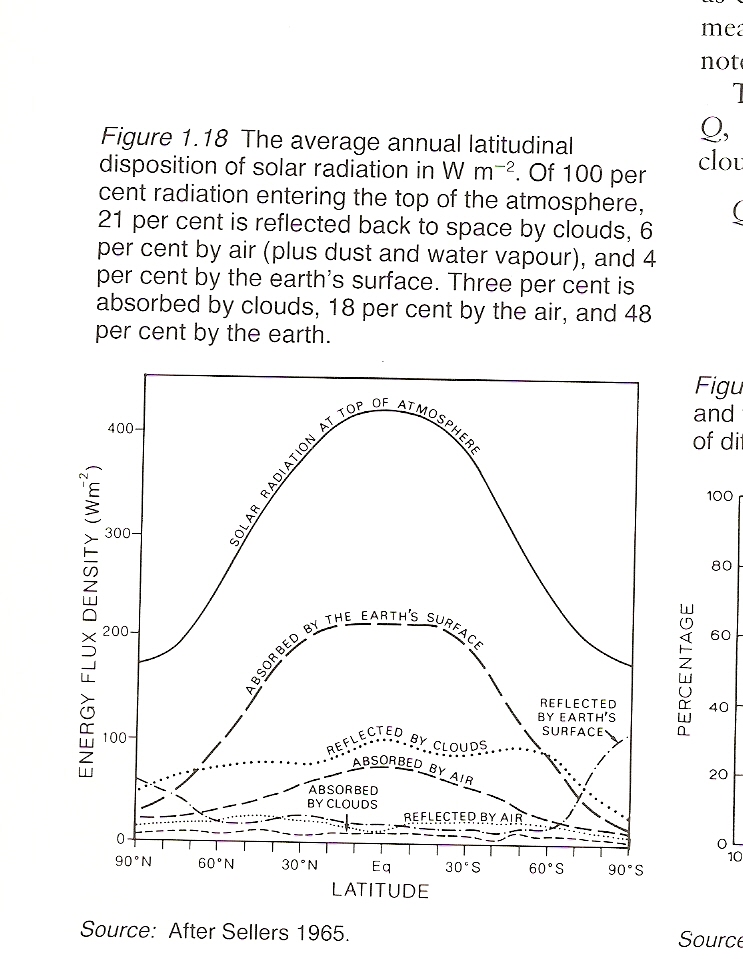
Chapter 4: A more detailed look at what happens to solar

energy as a function of latitude.

Chapter 4: What Makes a Gas a Good Greenhouse Gas?

1) It must have absorption lines at frequencies where the earth emits thermal energy. One reason why CO2 is a good greenhouse gas for earth is because it absorbs thermal energy at the peak of the earth's Planck function.

2) Are there other absorbers already present? If so adding additional absorbers at that frequency won't make much difference.

3) How much of the absorber is already there? The radiative forcing per molecule is highest when you first add it, then decreases as you add more and more.

4) How many absorption lines does the molecule have? More complex molecules will have more absorption lines (more ways to vibrate or rotate) so will be better greenhouse gases. CFC's are perhaps the prime example. On a per molecule basis their radiative forcing of CFC-11 is about 10,000 times that of CO2. It turned out that banning CFC's in the interest of ozone depletion has probably played some role in slowing down climate change in the past 2 decades.

5) The height the molecule being added. Generally, the higher the temperature contrast between the surface and the molecule (i.e. the ambient temperature at the emission height), the better a greenhouse gas the molecule will be.

Chapter 4: The Earth Energy Budget

Notice how the 9.6 micron O3 band and the 15 micron CO2 band give rise to increase absorption at these wavelengths. Notice also that wavenumbers lower than 2000 cm-1 are in the LW part of the spectrum, so the plot above is entirely LW. Note that rapid increase in absorption as you go lower than 0.32 microns. This is due to the absorption of UV light by ozone.

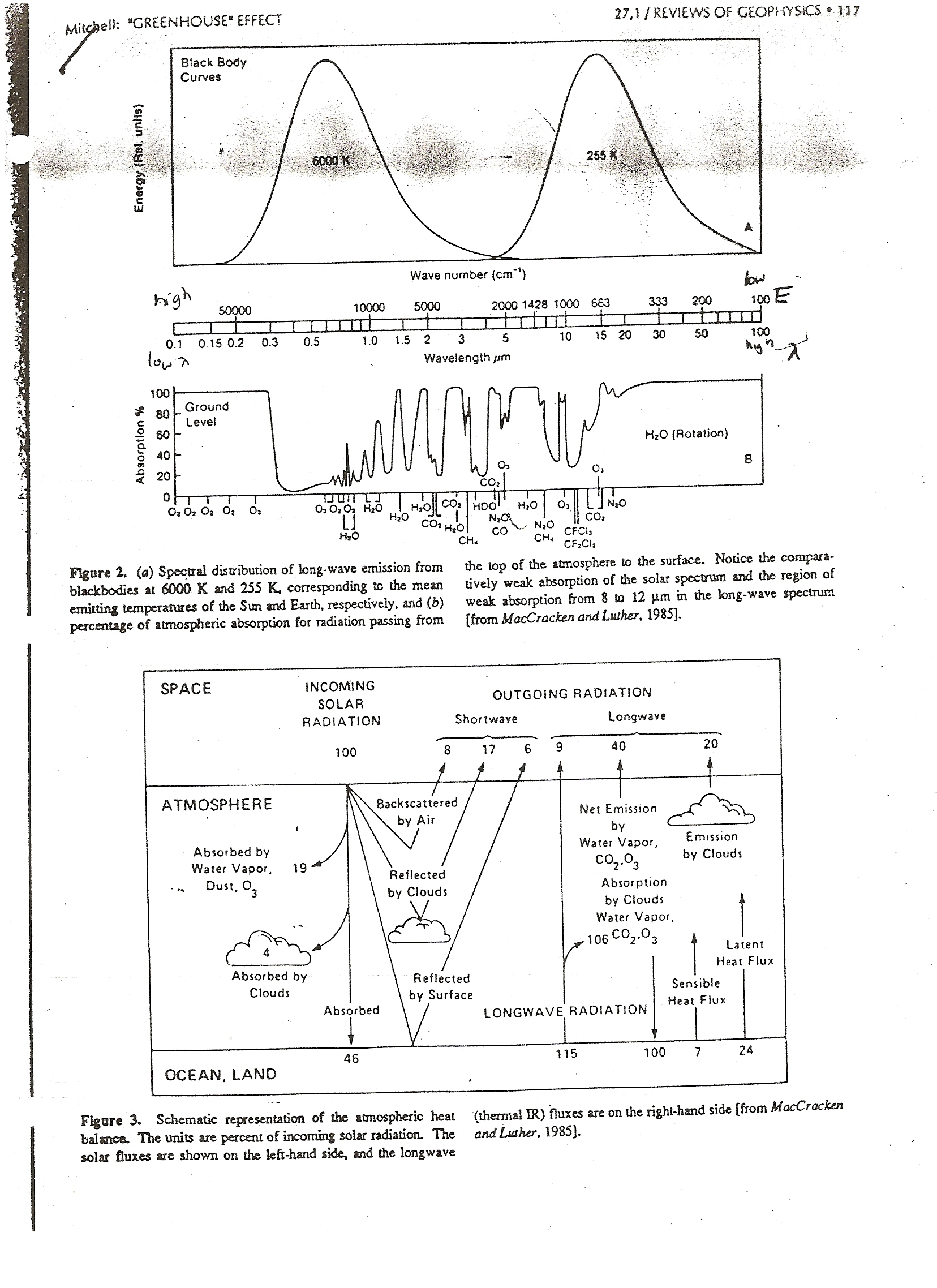
You should know how to use this lower plot to estimate the solar reflectivity of the earth, the solar absorptivity of the atmosphere, and the long wave emissivity of the atmosphere. Note that 100 incoming solar units equals a global average of 340 W/m2, so to convert from the units here to W/m2, multiply by a factor of 3.4.

Chapter 4: Earth Energy Budget Plot - in W/m2

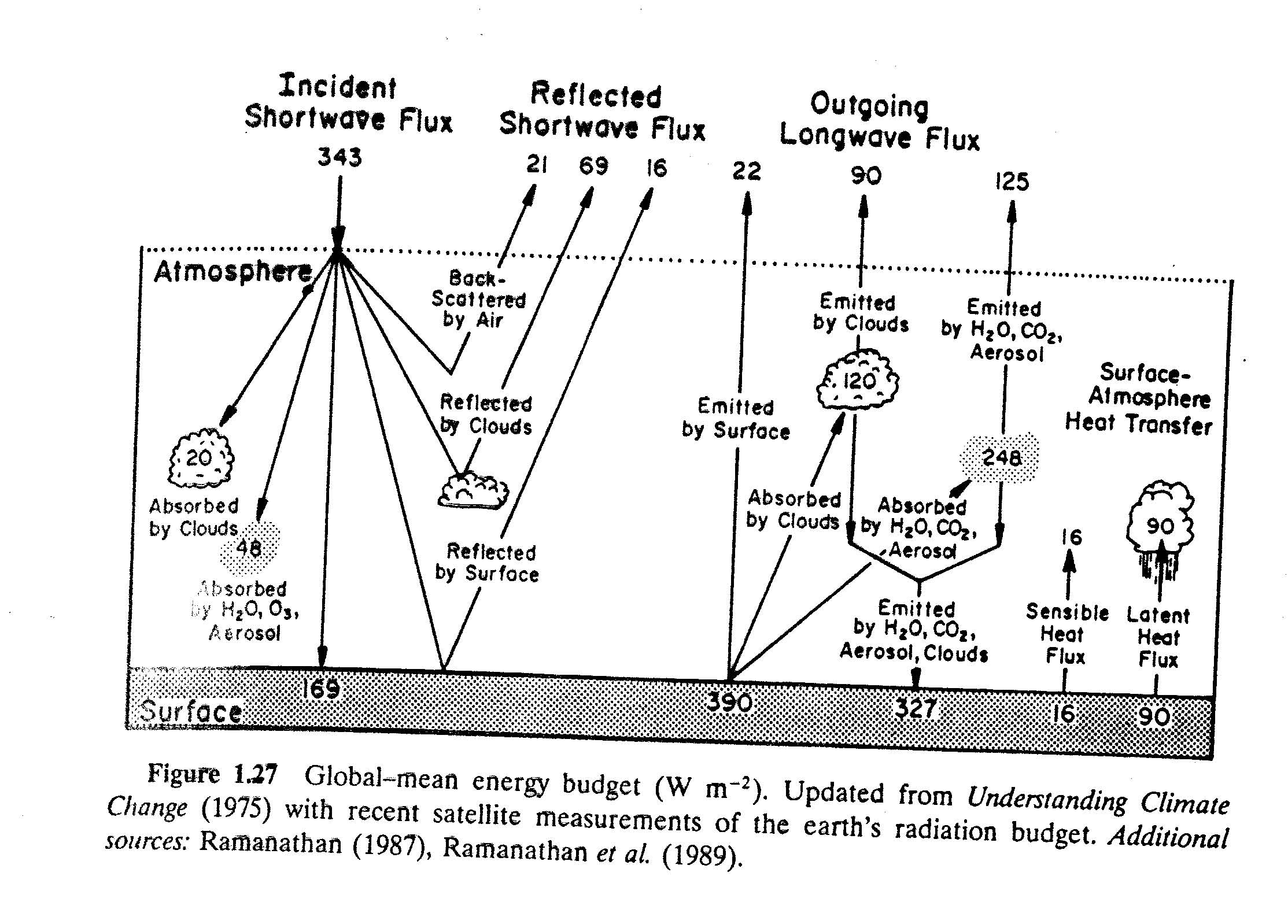
In steady state, there must be a balance in 3 distinct energy budgets.

(1) TOA Energy Balance:

Energy into the Planet from Space = Energy out from the Planet to Space.

SWin + LWin = SWout + LWout.

343 + 0 = (21 + 69 + 16) + (22 + 90 + 125)

343 + 0 = 106 + 237

(2) Atmospheric Energy Balance:

We also have to take into account the surface heat fluxes of heat to the atmosphere:

SWin + LWin + Sensible Heat Flux + Latent heat Flux = SWout + LWout

(20 + 48) + (120 + 248) + 16 + 90 = 0 + (90 + 125 + 327)

542 = 542

(3) Surface Energy Balance:

SWin + LWin = LWout + Sensible Heat Flux + Latent heat Flux

169 + 327 = 390 + 16 + 90

496 = 496

Chapter 4: SW versus LW

This difference is fundamental: SW photons come from the sun while LW photons come from an object on the earth. The average temperatures of the sun (6000 K) and earth (255 K) are so dissimilar, that their black body spectra have no overlap. If a photon has a wavelength larger than 4 microns, it is LW. If it's wavelength is shorter than 4 microns, it is SW.

It makes sense to talk about absorption and scattering of SW photons in the atmosphere. It does not make any sense to talk about emission of SW photons in the atmosphere: the black body emission spectrum of any object in the atmosphere is essentially zero at wavelengths less than 4 microns.

It makes sense to talk about emission and absorption of LW photons in the earth's atmosphere. We do not not usually talk about scattering of LW photons in the earth's atmosphere. Why? Mainly because the size parameter x is usually too small. A typical LW wavelength is perhaps 15 microns (near the peak of the earth's LW spectrum). Scattering could occur either via molecules (r ~ 1 nm, x ~ 0.0004), aerosols (r ~ 100 nm, x ~ 0.04), cloud droplets (r ~ 10 microns, x ~ 4), cloud ice crystals (r ~ 100 microns, x ~ 40), or raindrops (r ~ 1000 microns, x ~ 400). (See Figure 4.11 of the text for more details). LW scattering by molecules and aerosols does occur, but the small value of x makes the scattering efficiency sufficiently small that this process is not relevant to climate. LW scattering by clouds and ice crystals is of borderline relevance. Emission and absorption of LW energy in clouds is much more important. LW scattering by raindrops would be important when it is raining, but again, raindrops would be efficient absorbers of LW photons.

Chapter 4: Guam Spectral LW Emission Image

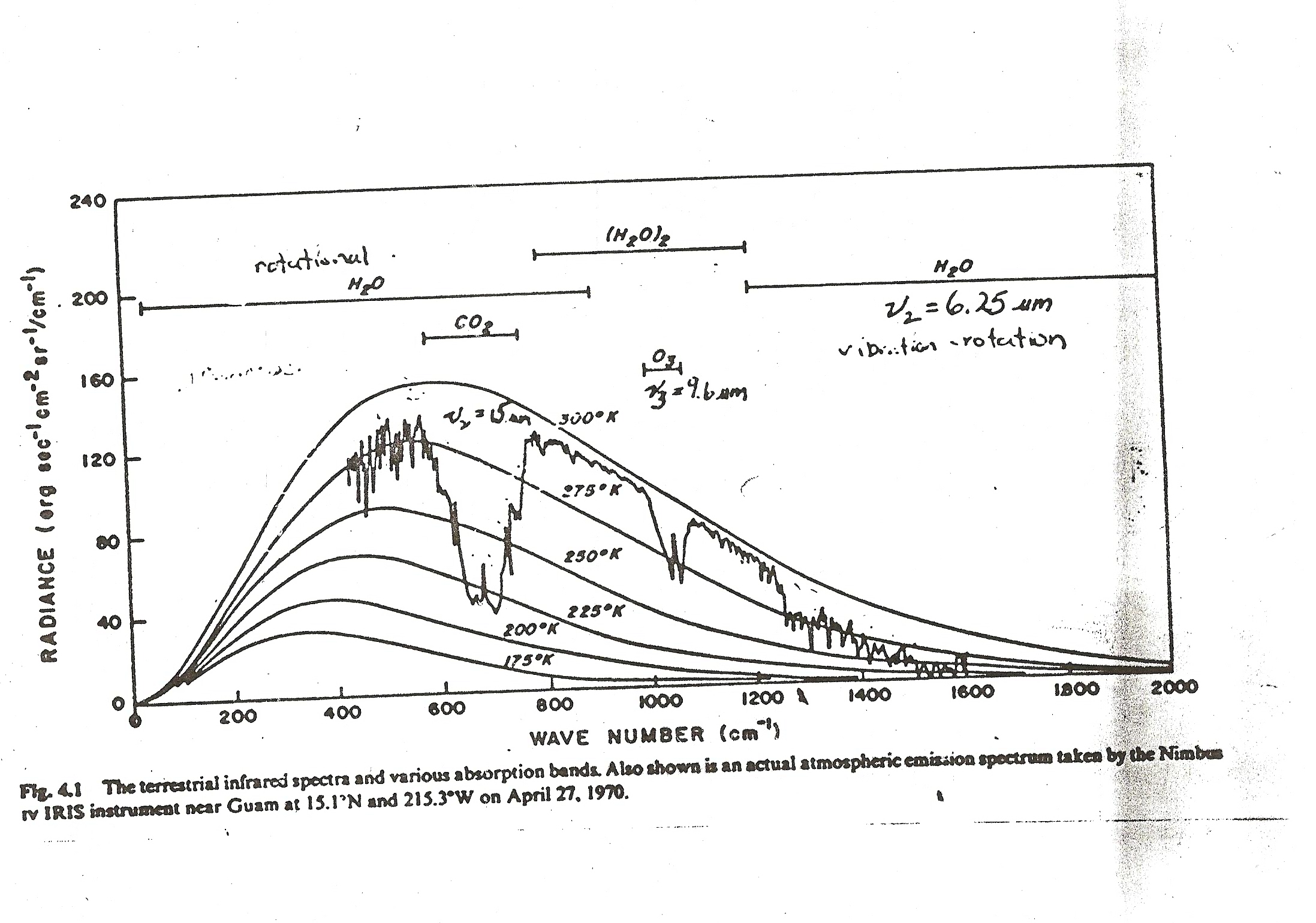
Notice that the horizontal scale is wavenumbers or cm-1. Small wavenumber corresponds to low energy, while large wavenumber corresponds to higher energy.

This plot shows the LW radiance a satellite would measure from space looking down at the surface, when no clouds are present, over Guam. In the absence of greenhouse gases in the atmosphere, the satellite would observe a black body curve close to 300 K (likely the approximate surface temperature). If you look at the so-called window region between 800 cm-1 and 1200 cm-1, this is approximately what you see. In this region, there are very few greenhouse gases that emit and absorb LW radiation - with the exception of ozone near 1050 cm-1 (or 9.6 microns).

Near their absorption bands, greenhouse gases absorb the warm radiation upwelling from the surface, and replace it by colder radiation of reduced intensity, corresponding to the local temperature at that height. The dominant absorption feature in this image is the 15 micron CO2 band. Most of this emission is coming from CO2 molecules in the upper troposphere and lower stratosphere. In the tropics, the average temperature of the tropical tropopause is about 195 K, so it is hard for the CO2 emission to go below the 200 K black body curve, even if most of the emission to space at a particular wavelength (dF_lambda/dz) is emitted from a height region close to the tropopause.

There is a narrow spike in CO2 at the center of the CO2 band. This occurs because, at this wavelength, where the absorption cross-section of CO2 is largest, most of the emission to space is coming from the stratosphere, where the temperature increases with altitude, and it is warmer than temperatures near the tropical tropopause.

The rotational and vibrational bands of water vapor are also clearly very important over a broad range of wavelengths.

Measuring the black body emission spectrum of a planet or star is a good way of getting insight into the composition of its atmosphere.

Chapter 4: LW Emission Spectra from Different Regions

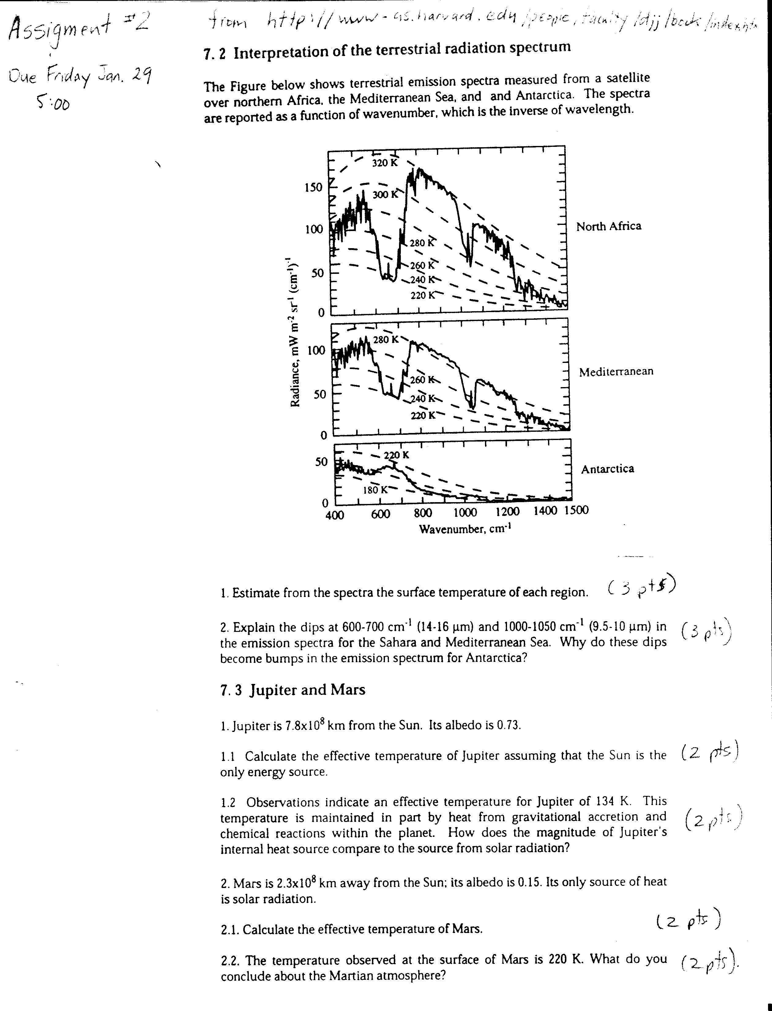
The LW emission spectra can vary dramatically depending on the surface temperature and whether clouds are present. This figure shows clear sky LW spectra from three regions. The surface of Antarctica appears close to 180 K (!). In this case, since the surface is so cold, CO2 is increasing the LW emission to space.

Given the value of the solar flux S0 of a planet, and its solar reflectivity, one can calculate its TE. An average surface temperature Ts > TE does not always imply that there is a greenhouse effect. The planet could have an internal heat source. For example, a large planet could be undergoing gravitational compression - this decrease in gravitational potential energy would be converted to heat. Another possible heat source is internal radioactive decay. On earth this is very weak, but significant since it maintains mantle convection, and the movement of tectonic plates and volcanism.

Chapter 4: LW Emission Spectra from a Cold Cloud

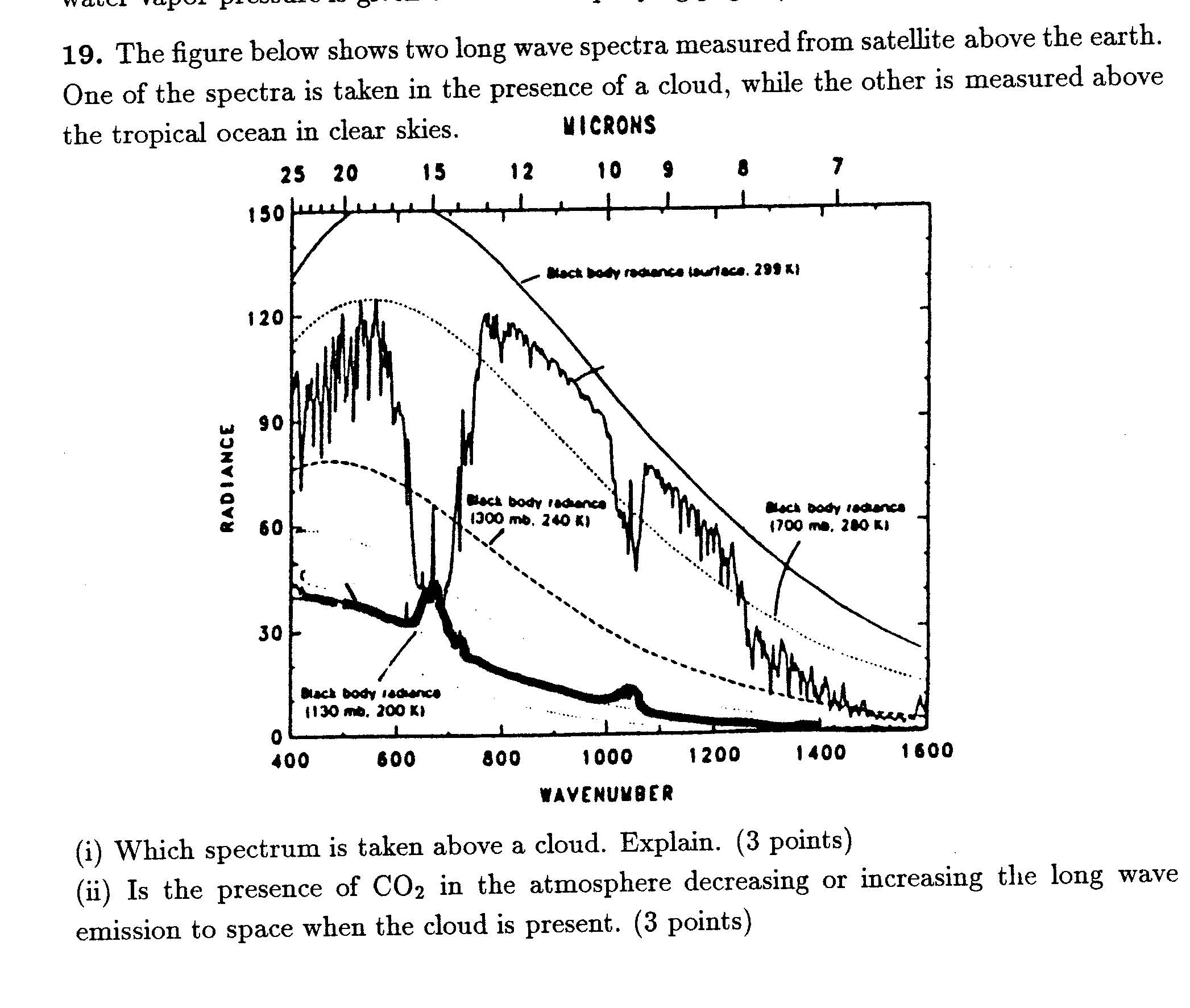
The LW emission shown as the thick line was taken when a cloud was present. The cloud is acting like a grey body (or close to a black body). There seems to be no trace of the warm LW emission from the surface. The cloud top is clearly significantly colder than 240 K, since it lies significantly below the 240 K dashed black body curve. Clearly, high cold clouds can dramatically reduce the LW emission to space, and be powerful greenhouse agents (acting like emergency blankets).

The peaks in the cloud spectra refer to LW emission from CO2 and ozone in the stratosphere. This emission is coming from a height range in the stratosphere which is warmer than the cloud top, so that CO2 and O3 are increasing the LW emission to space (functioning as anti-greenhouse gases in this instance).

Chapter 4: Absorption Lines

Some of the thermal radiation emitted by the surface goes directly to space, especially in the so-called "window" region. (But note that the atmosphere is only transparent to LW radiation in this wavelength region when no clouds are present.) Radiation at other frequencies (or wavelengths) is much more likely to be absorbed. Greenhouse gases absorb only at special frequencies (or wavelengths), corresponding to resonant energies at which they vibrate/rotate. These are called absorption lines. A satellite looking at the thermal radiation emitted by the earth sees decreases in radiance at these absorption lines. This is because the "warm" thermal radiation emitted from the surface is absorbed at these wavelengths, and is replaced by "colder radiation" (reduced radiance) coming mainly from gases in the atmosphere at a temperature colder than the surface. This reflects the insulating behavior of greenhouse gases.

In order for greenhouse gases to increase the surface temperature, the atmosphere must be colder than the surface. Otherwise greenhouse gases would increase the emission of thermal energy to space. For example, there can be no greenhouse effect on a planet with an isothermal atmosphere.

Greenhouse gases emit and absorb LW radiation only at very specific frequencies or lines. However, in the liquid or ice form, as in a cloud, water becomes a grey body and has an emissivity which is only weakly wavelength dependent. This is a deeply strange result: why would a water molecule behave so differently depending on whether it is in the gas phase or a liquid? Perhaps the easiest way of explaining this is that the energy levels of water molecules are smeared out by the closer presence of the other water molecules in the liquid or ice phase, so they are no longer independent oscillators (springs), but can interact with the radiative field at a continuum of energy levels.

Chapter 4: What is cloud Liquid Water Path (LWP)?

Cloud LWP is the depth of the puddle of water you would make by collecting all the cloud droplets together. Most clouds do not contain very much water. In fact non-precipitating clouds typically have an LWP of 0.1 mm. This is remarkably small, and demonstrates that dividing liquid water into tiny droplets can greatly magnify the scattering of visible light by the cloud. Precipitating clouds can have much larger LWP's.

Chapter 4: Factor of 4 in S0/4

The area of the sun's radiation that the earth intersects is pi times the radius of the earth squared. The total area of the earth is 4 times pi times R squared. The global 24 hour average TOA (Top Of the Atmosphere) solar flux is therefore S0/4. In constructing a simple one layer climate model, all fluxes have to be global averages. Therefore, S0/4 is the appropriate TOA solar flux.

However one does not always automatically divide S0 by 4 in every case. In the case of a directly overhead sun, the TOA solar flux is S0. In the case of solar zenith angle of theta, the TOA solar flux is S0 times cos(theta). Try and determine from the question whether is is based on a particular solar zenith angle theta, or is a climate type problem where it is more appropriate to use S0/4 (i.e. globally averaged as opposed to instantaneous values of solar flux).

Chapter 4: One Layer Grey Atmosphere Toy Model

If a planet did not have an atmosphere, and no internal heat source, its average surface temperature would equal its TE ( = 255 K for the earth). The purpose of this model is to show that an atmosphere with greenhouse gases will give rise to a surface temperature Ts > TE, and a atmospheric temperature Ta < TE.

The main defect of the One Layer model is that it over predicts the surface temperature, since it does not consider solar absorption in the atmosphere.

The Global Energy Budget Figure shows that 106 of the upwelling 115 units of LW radiation from the surface is absorbed in the atmosphere. This gives a LW absorptivity due to greenhouse gases and clouds of 0.92. The one layer model (with no solar absorption in the atmosphere) predicts that the mean surface temperature of earth in this case should be 297 K. The actual global mean temperature is 288 K, so this model overestimates the surface temperature by 9 K.

The main reason for the overestimate is that the One Layer model assumes that all solar energy not reflected to space is absorbed at the surface. Figure 3 shows that 46 units of solar energy are absorbed at the surface and 23 in the atmosphere. Solar absorption in the atmosphere increases the temperature of the atmosphere, and therefore decreases the effectiveness of greenhouse gases.

Solar absorption in the atmosphere also decreases rainfall, by making the atmosphere more stable - it is harder for clouds to rise up through a warmer atmosphere.

Chapter 4: Spectral response to Doubling CO2

FIXED RESPONSE:

If you double the concentration of CO2 in the atmosphere, but keep everything else about the atmosphere fixed (clouds, water vapor concentrations, the surface temperature), you will reduce the outgoing LW flux to space by about 4 W/m2. The top plot gives an idea of the wavelengths (or wavenumbers) at which this reduction in LW flux is coming from. It represents the change in the LW emission to space from a CO2 doubling as a function of wavelength. The center of the CO2 band is 750 cm-1. Doubling CO2 in a fixed atmosphere decreases CO2 emission at most wavelengths in the band, as you would expect, but increases CO2 emission at the center of the band. Why?

At any wavelength, doubling CO2 increases the effective height of average emission to space at that wavelength, i.e. moves the peak of the weighting function to a higher altitude. At the center of the band, where the absorption coefficient of CO2 is largest, the height of maximum emission to space is occurring at the highest altitude. This wavelength is labeled "1" to be consistent with the notation of Figure 4.33. At this wavelength, where the absorption cross-section of CO2 is largest, the CO2 emission to space is not coming from the troposphere, but from the stratosphere where temperatures increase with altitude. Figure 4.33 shows that this weighting functions peaks near 30 hpa, or 25 km. The emission to space at the center of the CO2 band will increase when CO2 is doubled because this emission will now come from an even warmer temperature (i.e. at an even higher stratospheric altitude). At the sides of the band, where the emission is coming from the troposphere, increasing the average height of emission reduces the average emission temperature and reduces the intensity at these wavelengths.

If you were to average over all wavelengths, you would get an overall reduction in LW radiation to space (~ 4 W/m2) from doubling CO2 in a fixed atmosphere. This is an integral over the center of the band where emission is increased, and at the sides, where emission is reduced. This reduction in LW emission causes an energy imbalance in the earth: total emitted LW to space from the earth is no longer equal to the total absorbed SW by the earth. The lower figure shows how the atmosphere responds to this imbalance.

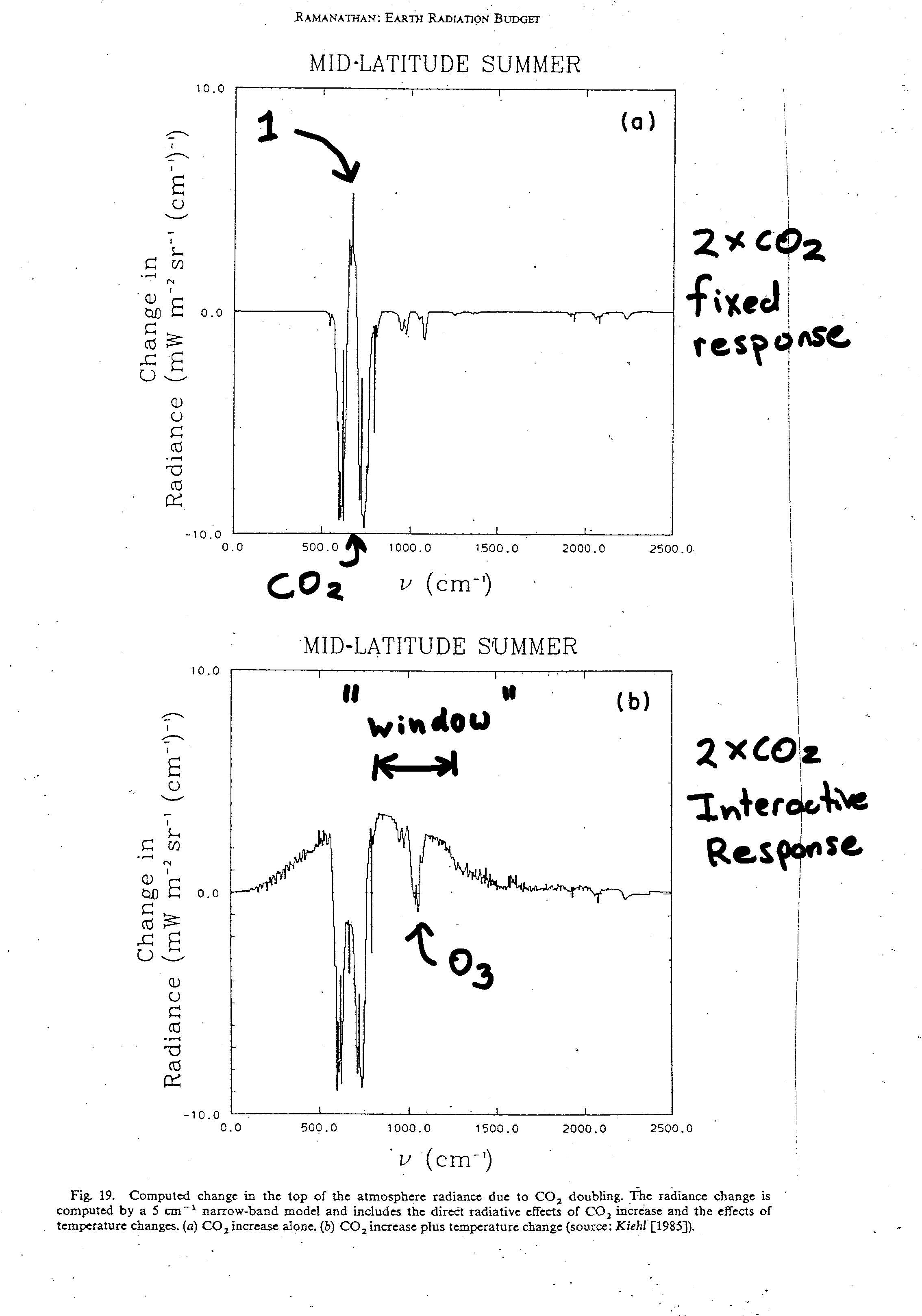
INTERACTIVE RESPONSE (Could also call Steady State Response):

The climate system must respond to any energy imbalance. The lower plot shows how the LW emission to space changes in response to the atmospheric changes triggered by an energy imbalance from a CO2 doubling. Surface and atmospheric temperatures and water vapor concentrations have been allowed to change in such a way to reach a new energy balance. The stratosphere clearly cools: The LW emission at the center of the CO2 band goes down. This is driven by an increase in LW cooling in the stratosphere due to the increased CO2 (see explanation below). Unless this increased LW cooling were somehow compensated by an increase SW ozone absorption, stratospheric cooling must occur, and it does (both in this model and the real atmosphere).

There is increased emission to space in the window region between 750 and 1500 microns (except for the ozone band in the middle). This is the region where, in the absence of clouds, the atmosphere is quite transparent to LW radiation, so that the LW intensity to space is a direct indication of surface temperatures. By increasing the surface temperature, and increasing the LW emission to space in the window regions, the earth is trying to compensate for the reduced LW emission to space within the CO2 band. Provided there is no change in solar absorption, the change in LW radiance integrated over all wavelengths must be zero to maintain energy balance: if you integrate the change in radiance over all wavelengths in the lower plot, you should get zero. The window region functions as the earth's radiator fins. They are the way the earth can directly get rid of excess energy by warming the earth's surface (Of course these radiator fins are prevented from working when there are clouds.)

This figure helps demonstrates the importance of stratospheric cooling to the greenhouse effect: if the stratosphere did not cool, so that doubling CO2 increased LW emission to space from the stratosphere, you would not need as much surface warming to bring about a new energy balance.

Chapter 4: Why are increased CO2 concentrations expected

to continue to cool the stratosphere?

Stratospheric temperatures have been decreasing for several decades. This is consistent with an increased greenhouse effect. Why?

From the energy budget figure above, the atmosphere absorbs 106 units of LW radiation but emits 160. This 54 of net LW atmospheric cooling is balanced by 7 units of sensible heat flux, 24 units of latent heat flux (condensational heating), and 23 units of solar absorption. Solar absorption is therefore a significant term in the energy budget of the atmosphere, especially in the stratosphere where condensational heating is zero, and there is a direct balance between solar absorption and net LW emission. The main solar absorber in the stratosphere is ozone. Water vapor concentrations in the stratosphere are extremely low, so that the main greenhouse gas is CO2. Increasing CO2 increases the rate of LW cooling. In the absence of any way of increasing the SW heating rate, the only way for the atmosphere to maintain energy balance is to reduce temperatures in the stratosphere.

In the above calculation, the solar absorption "a" in the stratosphere is due to ozone. The observed stratospheric cooling is therefore likely due to some combination of ozone depletion and CO2 increases, but the dominant reason for the temperature decrease would be the CO2 increase.

It might strike you as inconsistent that increasing the concentration of a greenhouse gas tends to cool the atmosphere (increasing LW emission) but warms the surface. But actually, this is quite consistent. If you wear a winter jacket, you want it to be well insulated so that your body heat does not easily diffuse to the outside surface of the jacket. By keeping the outside surface of the jacket cold, you reduce LW emission to your surroundings, and stay warm.

Chapter 4: Absorption coefficient = Emission coefficient

This only applies to greenhouse gases and clouds in the LW part of the spectrum. For example, the LW emissivity of a cloud will equal the LW absorptivity of a cloud, but will not equal the SW absorptivity of the cloud. Also note that Kirchoff's law does not imply that the LW flux emitted by a cloud equals the LW flux absorbed by a cloud. It refers to the coefficients (emissivities) only.

Chapter 4: The Enhanced Greenhouse Effect (2 X CO2):

Suppose that the concentration of CO2 in the atmosphere were to double. On average, one would expect the longwave emission that reaches space from emission from CO2 molecules in the atmosphere to originate, on average, from a higher altitude. In general, temperature decreases with altitude. Increasing CO2 therefore tends to reduce the emission of longwave radiation to space (all other factors being equal). This "no feedback" reduction in outgoing thermal radiation to space has been calculated to be 4 W/m2 (using complex radiative transfer models of atmospheric emission, absorption, and scattering). In the absence of any change in the solar budget (i.e. no change in the solar reflectivity of clouds), thermal and solar budgets would be out of balance. There would be more SW energy coming in than LW energy going out. The only way to bring the LW and SW budgets back into balance is to increase the surface temperature. This also increases the temperature of the atmosphere (since the lapse rate of the atmosphere remains approximately moist adiabatic, at least in the tropics), so that LW emission from the surface and atmosphere both go up.

A radiative flux of 4 W/m2 is the amount of heat you feel standing about a 1.1 meters from a 60 W light bulb. What would happen if you REMOVED all CO2 from the atmosphere? Would you INCREASE thermal emission to space by 4 W/m2? No. It turns out that the radiative forcing of CO2 is highly nonlinear. Removing all CO2 from the atmosphere would actually increase outgoing thermal by around 25 W/m2!! This would cause a huge catastrophic surface cooling, as the surface temperature reduced in an attempt to bring the global energy budget back into balance (likely a snowball earth). And this calculation does not even take feedbacks into consideration. In general, the radiative forcing of a greenhouse gas depends non-linearly on its atmospheric concentration. When the gas is already present in high concentrations, adding more makes less difference. The absorption lines become saturated, and CO2 has a smaller climate impact. This is shown by the first two figures below in the Climate Dynamics Chapter.

Why do atmospheric scientists often prefer to associate the effect of a greenhouse gas concentrations with a change in radiative forcing, as opposed to a change in surface temperature? (i.e. doubling CO2 reduces LW emission to space by 4 W/m2). The radiative forcing of a greenhouse gas is the effect of a gas on the outgoing thermal radiation calculated by keeping atmosphere fixed at its current state. This "no feedbacks" calculation is quite unambiguous and straightforward. Scientists can agree on it, since we can agree how LW radiation propagates through the atmosphere. The actual effect of some change in greenhouse gas concentrations on surface temperature, after you have included feedbacks, is complex, and model-dependent, mainly because climate scientists have so many problems dealing with clouds. Hopefully some of these model uncertainties will diminish over time.

One way of viewing the greenhouse effect: provided the energy from the sun doesn't change, and the solar reflectivity of the earth doesn't change, the net thermal emission to space by the earth (combined surface and atmosphere) can't change. This implies that the net area under the curve shown in Figure 2.4 (Guam) can't change (treating it as if it were representative of a global average). If the level of CO2 in the atmosphere is increased, outgoing radiance within the 15 micron absorption line is reduced. To keep the net LW emission to space constant, this means that the outgoing radiance at other wavelengths must increase. It can most easily do this at wavelengths in the window region where the thermal radiation goes directly to space without being absorbed by the atmosphere. Since radiation in this window directly reflects surface temperature, an increase here implies the surface temperature is also increasing.

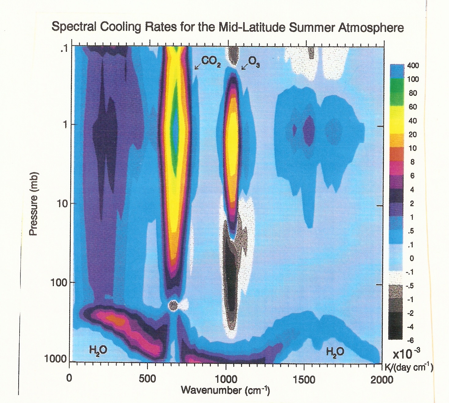
Chapter 4: Spectral Cooling Plot

This figure shows the importance of CO2 and O3 LW cooling in the stratosphere, and also that water vapor dominates in the troposphere (below 200 hPa). The 15 micron (800 cm-1) CO2 band dominates in the stratosphere. The 9.6 micron (1000 cm-1) ozone band also plays a role. Keep in mind 1 mb = 1 hPa, and 100 hPa is close to 16 km, 10 hpa close to 32 km, and 1 hPa close to 50km. Notice that there are altitude regions where CO2 and O3 actually heat the atmosphere locally (the grey regions where there is a negative cooling). These are height ranges where the local temperature is very cold, so that LW emission is reduced. Net absorption of LW radiation from below is larger than upward and downward emission, so there is a net warming.

This plot should be compared with Figure 4.29 in the text. Note for example, from Figure 4.29 that ozone gives rise to a LW heating between 150 hPa and 10 hPa. This is roughly consistent with the pressure range shown in grey for ozone in the plot below (grey in the image below corresponds to a negative cooling, i.e. heating.)

Chapter 4: Weighting Functions

This discussion is intended to provide some context to Figure 4.33.

Suppose a satellite is measuring the upwelling LW radiance from the earth at a particular wavelength. If this wavelength is within an absorption band of a greenhouse gas, then the photons reaching the satellite will be coming from the atmosphere, but possibly also from the surface as well, depending on the strength of the absorption line, and the concentration of the greenhouse gas. This is expressed in Eq. (4.48).

The first term on the left is Bi(Ts)*exp(-tau). Bi(Ts) is the black body emission from the earth's surface, while exp(-tau) is the probability that a photon emitted from the surface will reach space, or the transmissivity at that wavelength.

The second term on the right of (4.58) represents atmospheric emission reaching space, integrated over all altitudes. It is the product of a weighting function w(z) and the blackbody emission at that height B[T(z)]. The weighting function gives an idea of the relative importance of a height range to the intensity as measured by a satellite. By comparing the two lower plots of Fig 4.33, you can see that the weighting functions go to zero as the transmissivity exp(-tau) at that wavelength goes to zero. For example, the photons in band 1 measured by the satellite must all have originated above 200 hPa. Weighting function 1 peaks near 20 hPa (~ 25 km). Weighting function 2 peaks near 50 hpa (~ 20 km). Both peaks lie in the stratosphere, where the temperature increases with altitude. The intensity at wavelength 1 as measured by the satellite must be higher than the intensity measured by the satellite at wavelength 2, since it is coming from a height range where the atmosphere is warmer.

Transmission Probability: In the atmosphere, every CO2 molecule is continuously absorbing ambient LW radiation at wavelengths near its absorption lines. It is also emitting LW radiation at its absorption lines, at a rate depending on its local temperature. Photons emitted by CO2 molecules higher up in the atmosphere have a greater probability of reaching space than those emitted lower down. The transmission probability T(z) - the fraction of the photons emitted by CO2 which reach space from a given height z - will reach 1 at the top of the atmosphere, and progressively decrease as you approach the surface. The plot on the bottom right of Figure 4.33 shows how the transmissivity T(z) depends on wavelength as the the absorption coefficient of CO2 is increased from 1 - 6.

The mixing ratio of CO2 is roughly independent of height in the atmosphere (now about 380 ppmv). The total molecular density of air decreases exponentially with height - air gets thinner as you go higher up. This means that the CO2 density decreases approximately exponentially with altitude (even though the mixing ratio is constant). This is why all the weighting functions got to zero at high altitude.

Chapter 4: Increasing the CO2 Concentration moves the

peaks of the weighting Functions to a higher altitude.

Weighting functions go to zero at high altitude because the concentration of the greenhouse gas gets very small as the atmosphere becomes very thin. Increasing the concentration of a greenhouse gas therefore increases the value of its weighting function at high altitudes. Weighting functions tend to go zero as you approach the surface because the transmissivity is going to zero. Increasing the concentration of a greenhouse gas decreases the transmissivity even more, therefore reducing the weighting functions at low altitude. The combination of the high altitude increase + low altitude decrease shifts the weighting function to a higher altitude.

Chapter 4: Optical Depths in the Visible/UV

The vertical axis is optical depth from the Top of the Atmosphere (TOA) to the surface (sometimes called optical thickness). Note that the scale is logarithmic. If tau is less than 0.1, one considers the atmosphere to be basically transparent, if tau is between 0.1 and 2, the atmosphere is partially transparent, whereas if tau is larger than 2, the atmosphere is essentially opaque at that wavelength.

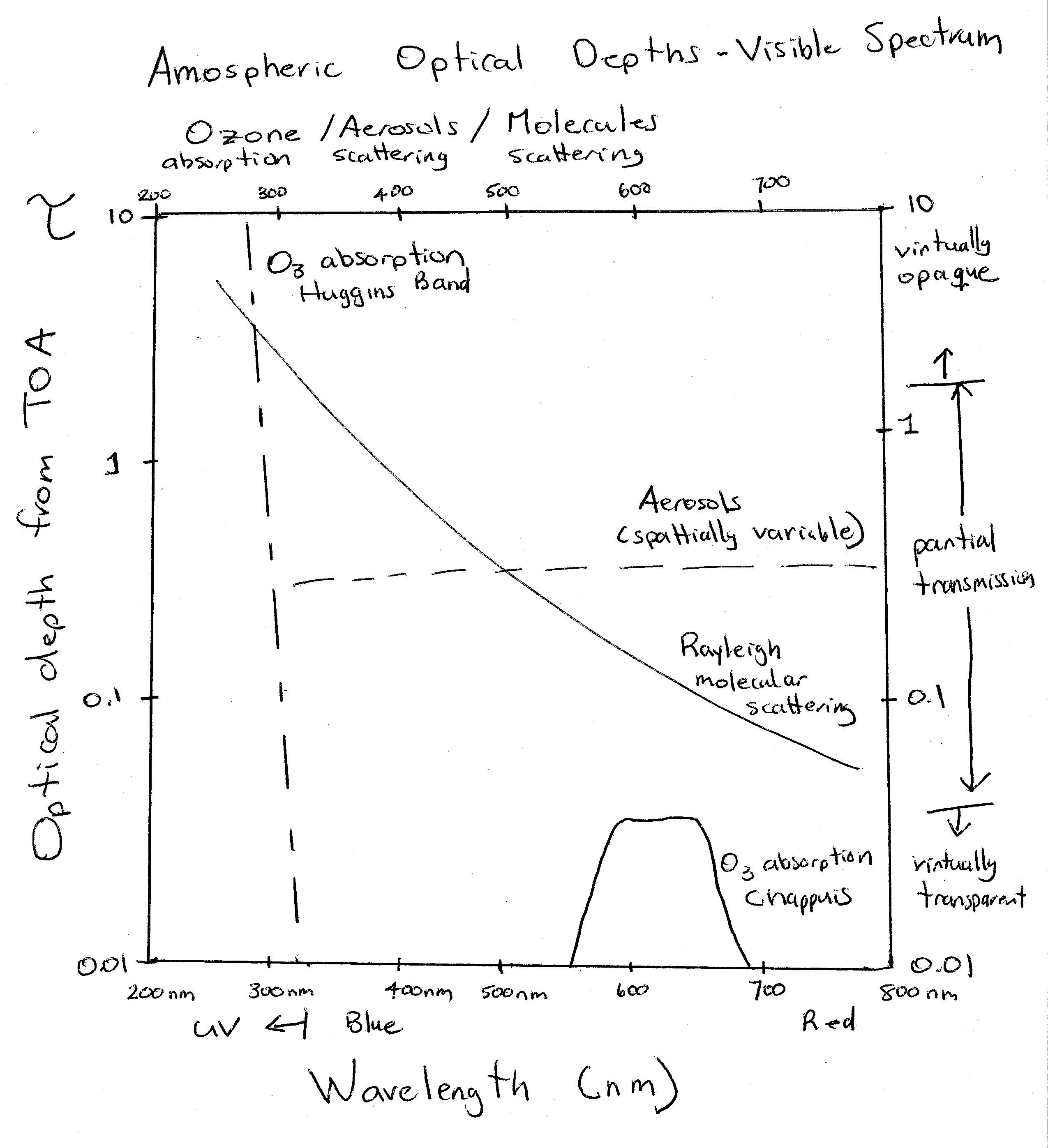
Molecular: Rayleigh scattering has the classic 1 over lambda to the fourth power dependence. The optical depth of Rayleigh scattering would depend on solar zenith angle - i.e. smaller for overhead sun than a sun lower in the sky. This plot would assume a particular Solar Zenith Angle (SZA); not sure what it is. The visible range is 380 nm to 780 nm. Our eyes have evolved to detect radiation in the maximum in the solar output of the sun since that is where the "signal" will be largest. It would be harder to see at 200 nm since there are so few photons at that wavelength, even though each photon would have a higher energy. The increased scattering of molecules in atmosphere at the blue (high energy) end of the visible spectrum makes the sky blue.

Ozone: The ozone absorption cross-section increases rapidly below 330 nm, so that by about 310 nm, ozone absorption is more important than molecular scattering in protecting us from UV light. It turns out that ozone is also a weak absorber of red light - the so called Chappuis band. Because this is weaker than Rayleigh scattering, it does not have much impact on the colour of the sun. The sun is yellow rather than white (its color in outer space) mainly because blue light is preferentially removed by molecular scattering.

Aerosols: The dashed line represents the scattering optical depth of aerosols. Aerosols both scatter and absorb solar light, but mostly scatter, unless they are very dirty, e.g. contain lots of soot. Aerosol scattering is highly variable in space and time; much higher in polluted regions, along the coast where there can be lots of sea salt aerosols, or downwind of forest fires. Note that the aerosol scattering is only weakly wavelength dependent. Aerosol scattering will therefore usually make the sky look white. This will be true unless the aerosols are very monodisperse - i.e. all have almost the same size, in which they can have a particular color.

Chapter 4: Scattering efficiency

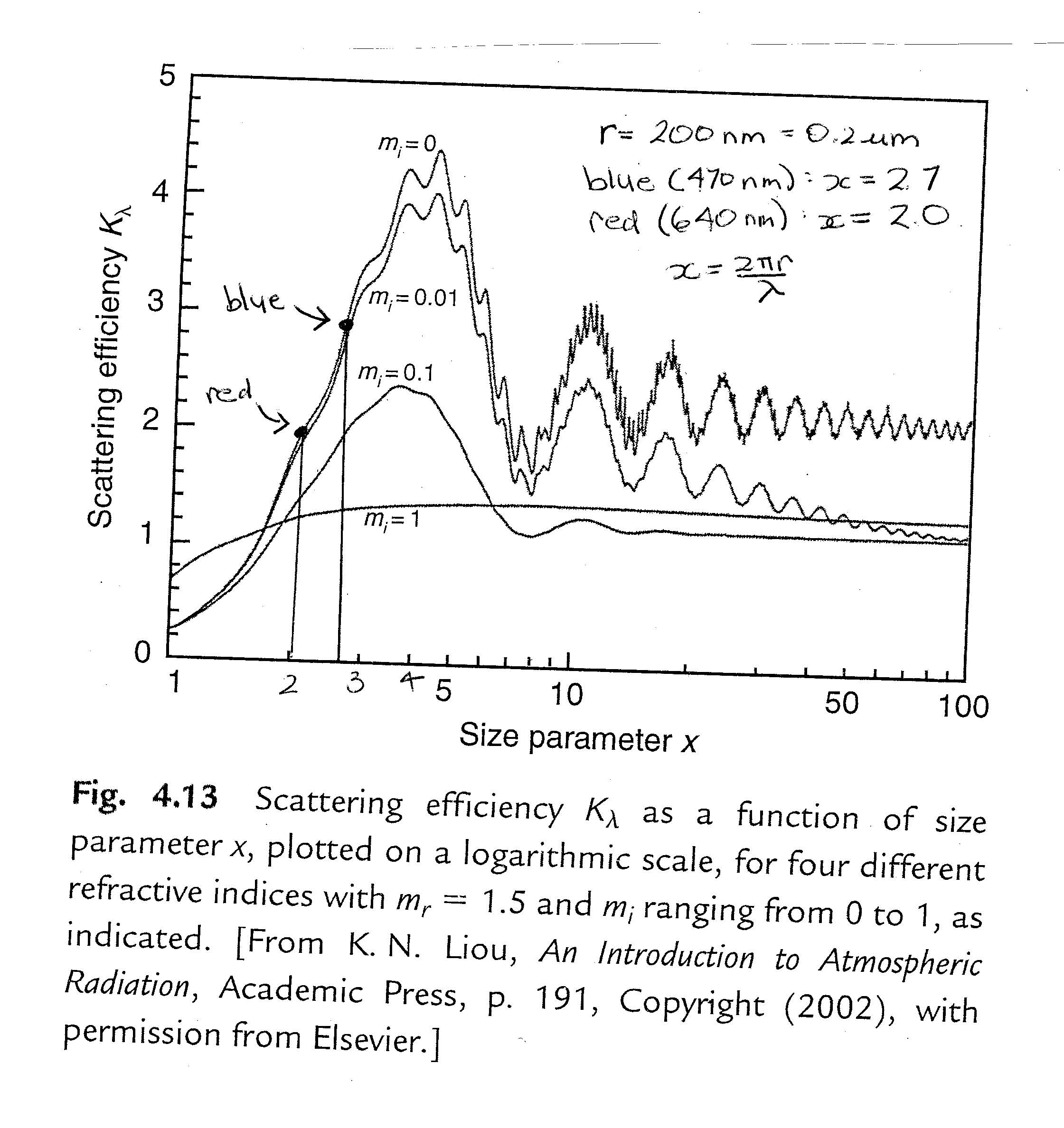
The fundamental definition is (4.16). It can be thought of as the probability of an incident photon being scattered, where incident refers to photons whose path intersects the areal cross-section of the aerosol (or molecule). The areal cross-section is just a way of expressing the physical size of the object, e.g. 4 times pi times the radius squared for spherical droplets. You would think that this probability can never be higher than 1, but Figure 4.13 shows that it can be larger than 4. (strike you as weird? Just remember that photons are waves and can be deflected by objects that they don't "hit" ...). Also note that the scattering efficiency scales as the size parameter x to the fourth power for small x. This "Rayleigh regime" is not shown in Figure 4.13. The mass absorption coefficient and the scattering efficiency refer to the same physical quantity, but express it in different units.

Chapter 4: Why are aerosols (usually) white?

Figure 4.13 shows that the scattering efficiency is almost always a function of the size parameter x. This means that almost every object has a color: it will scatter some wavelengths more efficiently than others. The exceptions would be scattering objects with very large x (> 100), where the scattering efficiency converges to 2, or objects which are highly absorbing (mi > 0), like soot. In class, I showed that the size parameter x of cloud droplets in the visible spectrum (350 - 700 nm) is large: this is the main reason why clouds are "white".

Aerosol particles are much smaller than cloud droplets, with a typical radius of about 100 nm. Aerosols are produced by pollution, forest fires, ocean spray, etc. Suppose that an aerosol has r = 200 nm. Then for blue light (wavelength = 470 nm), x ~ 2.7, while for red light (wavelength = 640 nm), x ~ 2. The figure below shows that this aerosol would have a higher scattering efficiency for blue light than red light. A cloud of such aerosols would therefore look blue. This is sometimes true. Cigarette smoke can have a bluish tinge to it. But usually, aerosols look white. A deep blue sky is a sign of a very clean atmosphere with few aerosols. This is because, in the atmosphere, aerosols usually come in a variety of sizes. Therefore, for each color, you have to average the scattering efficiency over a variety of values of x. This tends to make the average scattering efficiency nearly the same for all colors, with the result that a group of aerosols looks white.

Supplemental Material for Chapter 10 - Climate Dynamics

Chapter 10: Climate Sensitivity

A climate with high sensitivity has a large temperature response to a forcing, i.e. one in which positive feedbacks dominate. You get a larger warming if you increase CO2 and a larger cooling if you decrease CO2. A climate with low sensitivity is one in which negative feedbacks dominate. You get a weaker warming if you increase CO2 and a weaker cooling if you decrease CO2. (I am using CO2 here as a shorthand for any forcing. However, CO2 is sometimes a feedback rather than a forcing, and can therefore also affect the climate sensitivity.)

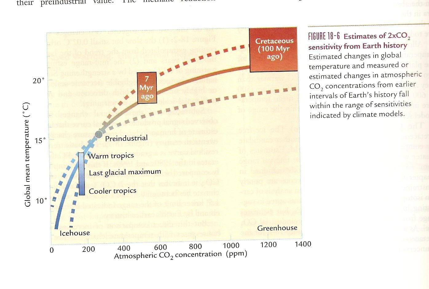
The Figure below shows that Paleoclimate evidence gives some guidance of the sensitivity envelope of the earth's climate, and therefore, the range of possible temperature increases we might experience as we increase CO2. However, there is no direct analogue of the current increase in CO2. CO2 changes during the Ice Ages were forced by changes in the latitudinal distribution of solar radiation at the earth's surface from changes in the earth's orbit around the sun.

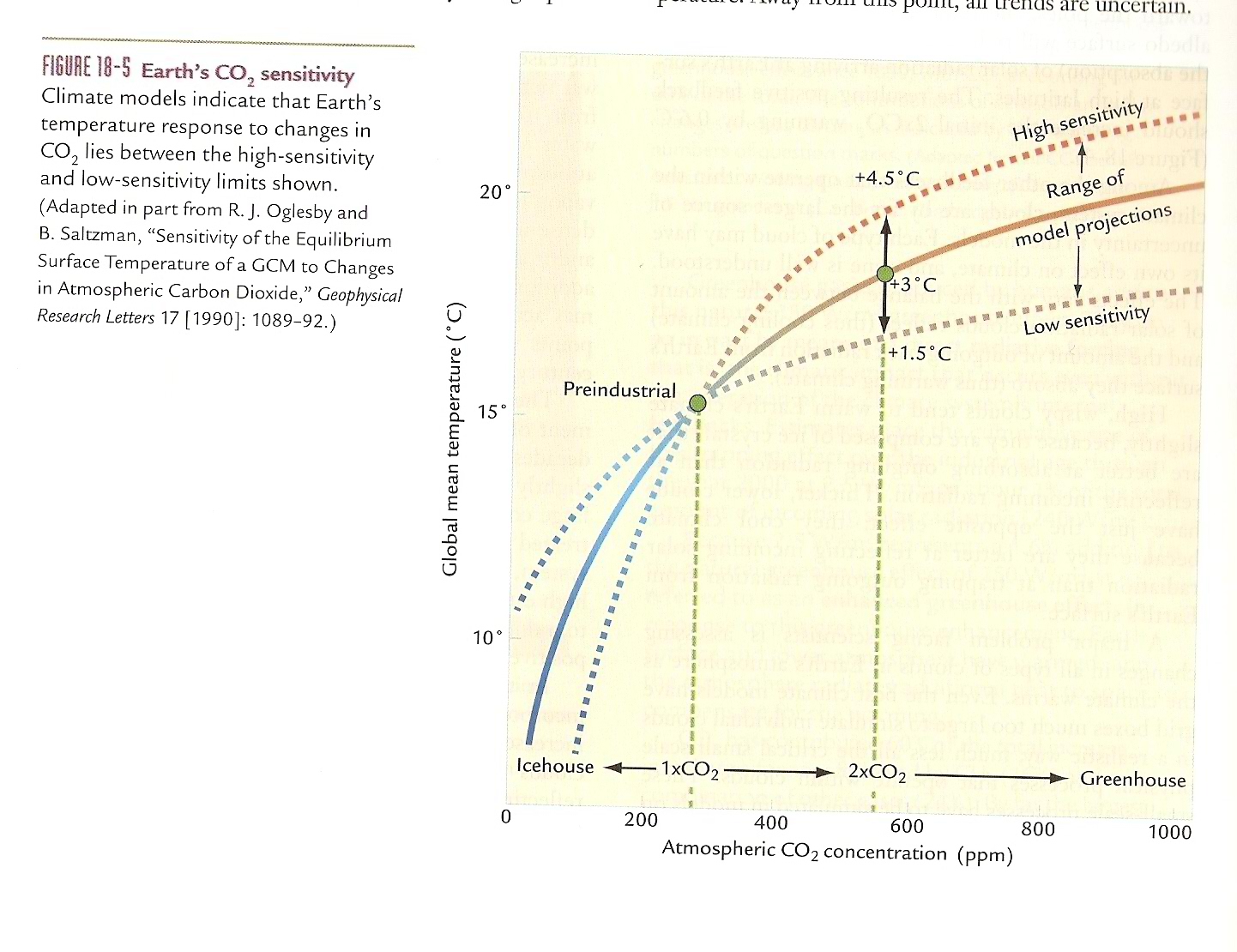
Chapter 10: Increasing CO2 is like going backward in time

The preindustrial concentration of CO2 was 280 ppm. It is now about 415 ppm, and increasing at about 2.5 ppm/year. To go back to the Cretaceous, we would have to burn all of our economically recoverable oil/gas and a lot of our coal. We would also have to sustain these high CO2 levels for at least several hundred years to allow the ocean to warm up, and the ice sheets to melt. Note the expected non-linear impact of CO2 changes on temperature. The term "Icehouse" is another word for a snowball earth. It is believed that the earth can revert to a snowball if CO2 levels in the atmosphere become sufficiently low (e.g. from reduced volcanic activity).

Chapter 10: How Climate Feedbacks Work

A radiative forcing is a process which changes the value of the LW flux emitted to space, or the amount of solar energy absorbed by the earth. A positive forcing would give rise to a reduction in the LW flux emitted to space (e.g. via an increase in the concentration of some greenhouse gas), or a decrease in the SW reflectivity of the earth. A negative forcing would be something that increases LW emission to space, or decreases SW absorption by the earth (i.e. volcanic eruption). The climate response induced by a forcing depends on "Feedbacks".

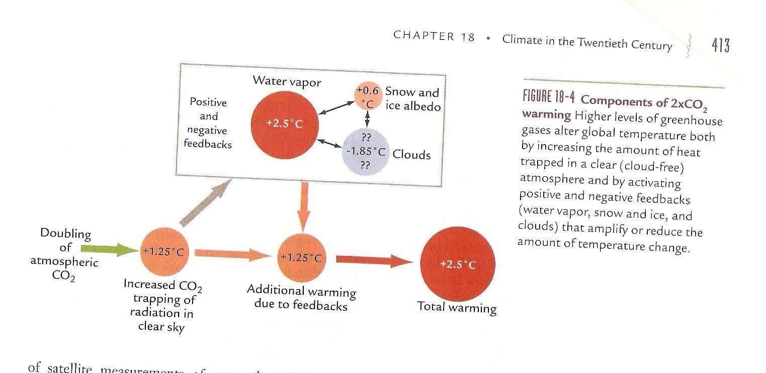
A doubling of CO2 would give rise to an initial decrease in LW emission to space of 4 W/m2. If the absorbed solar radiation remained constant, and there were no other changes in the atmosphere (water concentrations fixed, no changes in ice cover, clouds), there would have to be a surface temperature increase of about 1.25 C to bring the earth's energy budget back into balance. This 1.25 C increase is called the "No Feedbacks" response.

However, most models and the paleoclimate evidence suggest that the climate system has strong positive feedbacks. The two main positive feedbacks are the water vapor feedback, and the ice albedo feedback. This sign of the cloud feedback is not yet determined with certainty. However, the final steady state warming from these feedbacks likely gives rise to a temperature increase on the order of 2.5 C.

The main climate uncertainty is the role of clouds. How will the cloud distribution change in the future? Will the positive LW (greenhouse) forcing of clouds increase or decrease? Will the negative SW (solar) forcing of clouds increase or decrease? This is partly a cloud height problem. If average cloud height increases in response to a CO2 doubling, one would expect the cloud feedback to be positive. However, for example, if low-level boundary layer clouds or fog increases in response to a CO2 doubling, one would expect clouds to have a negative (stabilizing) effect on climate change. It is hard for climate models to simulate cloud cover accurately, since most clouds are so much smaller than the grid size of climate models (about 100 km).

Note that the sign of the overall current effect of clouds on climate does not determine the sign of the cloud feedback. For example, clouds in the current climate likely cool the earth when one considers both their LW and SW effects. However, this negative forcing could get smaller if you double CO2. In this case, the cloud feedback is positive, so it amplifies the climate response to any forcing.

An obvious similar case is snow and ice. Snow and ice increase the short wave (solar) reflectivity of the planet and therefore cool the earth. However, the ice-albedo feedback is positive.

The size of a feedback depends on the climate system. During warm periods in the past, where there was no ice or snow, the ice-albedo feedback would not have existed.

Examples of forcings: human induced emissions in CO2, changes in CO2 due to plate tectonics/volcanism, changes in the earth's orbit around the sun (tilt, eccentricity of orbit, etc), the solar cycle, volcanic eruptions. These changes drive climate change; they are not a response to climate change.

Chapter 10: Three Major Climate Feedbacks:

(i) Water Vapor (ii) Ice-Albedo (ii) Clouds

Ice-Albedo: Reductions in snow and sea/land ice cover are likely to amplify the warming especially in polar regions. This amplification is estimated as 20 %, globally, but is locally much more important in the Arctic, and is one of the reasons why the Arctic is expected to warm up the most. The size of the ice-albedo feedback depends on the amount of snow/ice present in the climate system. In a very warm climate regimes where there was none (e.g. 55 million years ago), the ice albedo feedback would not have existed. During ice ages this positive feedback would have much increased. This helped make the ice age climate more "noisy", e.g. millenial scale oscillations, Younger Dryas, etc. - although these temperature fluctuations may have been primarily caused by interactions of ice with the oceans, not purely ice-albedo feedbacks. Conversely the absence of an ice albedo feedback during warm regimes should have stabilized the climate.

Chapter 10: "Forcing" versus "Feedback"

The climate sensitivity is the change in surface temperature in response to some forcing, amplified or reduced by positive and/or negative feedbacks. In a given situation, how do you determine what is a forcing, and what are the feedbacks, since both the forcing and the feedbacks, in practice, are often changing together?

In the current climate, the CO2 changes are considered a climate forcing: they are not an internal response of the climate to something else. Orbital changes and volcanic eruptions are also examples of forcings. However, sometimes a change can be a forcing in one situation, but a feedback in another. The changes in ice volume during the ice ages were forced by orbital changes. However, CO2 tended to go down during the cold intervals and up during the warm intervals. In this case, the CO2 changes were acting like a feedback, and since they would have been amplifying the orbitally induced temperature changes, they would have been a positive feedback.

We don't have a very good understanding of why CO2 went down when ice volume increased, and vice versa. It probably had to do with an increased effectiveness of the biological pump during cold intervals.

The relationship between CO2 and temperature changes during the ice ages is not a good analogue for how we might expect current changes in CO2 to affect future climate: the ice age CO2 changes were a feedback response, whereas now CO2 is a forcing. However, the long slow tectonic decrease in CO2 over the past 100 million years was a "forcing".

Chapter 10: Hydrology of Berkeley and Halifax

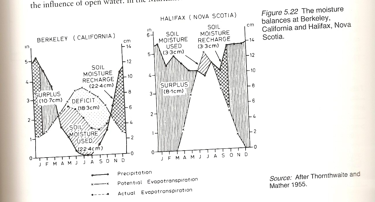
As I walk by the Halifax Citadel along Ahern street, you can almost always see drainage from citadel hill that spills over into the sidewalk and causes ice in the winter. Clearly, rainfall is exceeding evaporation on the Citadel, so that the citadel is a source of water to its surroundings almost the entire year. This figure shows that this is true generally of Halifax, with the exception of a few months in summer where evaporation temporarily exceeds precipitation. The rest of the time, the excess water flows out via rivers, streams, and gutters into the Atlantic. But this situation is relatively unusual. Most places in the world have a significantly longer season where the ground is in water deficit. This is especially true of places with Mediterranean climates like California, which receive most of their precipitation in the winter and very little in the summer. Hence they go into an extended period of water deficit in the summer, until the winter storage is used up and the soil becomes so dry that evaporation ceases. These types of places often require irrigation for agriculture. Although we have wet basements to worry about, we very rarely have water shortages ...

Chapter 10: Global Temperature Anomalies: 1850 - 2018

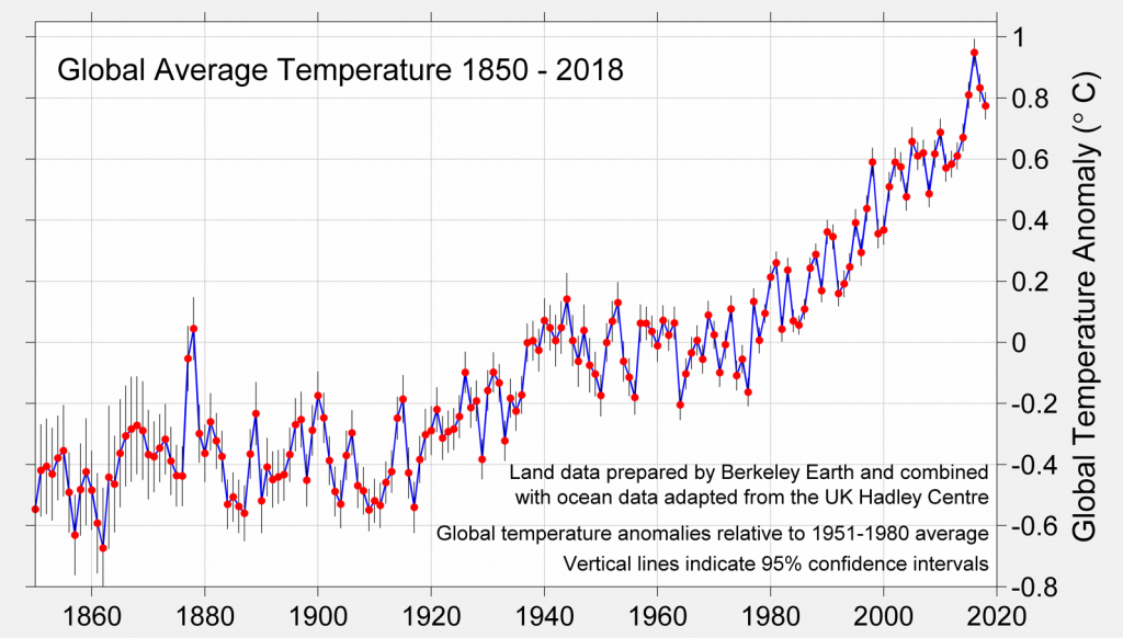
This figure shows that the earth has warmed up by about 0.8 C over the last 40 years, or about 0.2 C/decade. This rate of warming is roughly in line with the rate of warming climate models project will continue for the next 100 years (at present CO2 emission rates). The rate of global warming will likely accelerate if CO2 emissions go up, sea ice and/or Greenland ice goes down faster than expected (appears to be the case), and cooling from sulphate aerosols goes down (i.e. less burning of sulphur rich coal).

Also note that 1998 was about 0.2 C above the "normal" for that time, suggesting that the 1997/98 El Nino warmed the earth by about 0.2 C, about equal to one decades worth of current CO2 induced global warming. The reason an El Nino warms the earth is that the thick layer of warm water that builds up in the western Pacific during La Nina years spreads (sloshes) back the central and eastern Pacific. This increases global average SST's, which then increases temperatures in the global atmosphere (with some time lag of course). It is important to see the future global warming as a slow trend (on our timescales, fast compared with geological timescales), which is superimposed on faster natural variability. There is always a multiplicity of both natural AND human processes affecting climate, and it is extremely difficult to disentangle them. CO2 induced global warming can contribute to a trend in global temperatures but does not by itself help you understand questions like why 2007 might be colder or warmer than 2006. The year-to-year noisy interannual variability in climate will always be dominated by the ENSO phase, volcanoes, solar induced variability, other facts we do not understand, as well as just "chaos".

Chapter 10: ENSO

Note that El Nino and La Nina are just different phases of ENSO. ENSO is the name for the oscillation as a whole (as in "high index" is the name for the phase of the NAO when the Icelandic Low is deeper). In class, I sketched the positive feedback between the ocean and atmosphere that brings about an El Nino. But why does an El Nino end? In other words, why do the warmest SST's and rainfall go back to their normal configuration where they are highest in the Western Pacific? I don't really know the answer, but because we live on a rotating planet, the equatorward trade winds will be deflected to the west as they converge toward the equator, and this drives a westward surface flow along the equator in the tropical Pacific ocean. (Presumably, if the earth spun in the opposite direction, the highest SST's would occur on the eastern Pacific ....) One would therefore expect the "normal" configuration to have high SST's and rain in the western Pacifc, since that is the location where the surface ocean waters have been warmed by longest exposure to solar radiation. Perhaps an El Nino event tapers off when the anomalous warming of the surface ocean waters in the central Pacific diminishes. The cooler water would become less able to support convection (rain), and the trade winds would intensify as the convection in the Western Pacific increased. In the early stages of an El Nino event, the warmer water in the central Pacific would be maintained by a flow of warm water from the west. Once this wedge of warm water in the Western Pacific drains away (that had built up during the previous La Nina phase), and the flow stops, the warm water in the central Pacific would likely cool due to latent heat fluxes (i.e. the warm water is the source of the water vapor for the convection above it and this leads to evaporative cooling at the surface.)

Chapter 10: Climate Change and The Nature of Scientific

"Truth" (Not Required)

The case that humans are warming the climate arises from a variety of indirect lines of evidence: predictions of both simple and complex physical models, the observed surface warming over the past 100 years (and especially the last several decades when the observational record has been better), the ability of models to reproduce this warming as a response to changes in CO2 (with caveats related to uncertainties over boundary conditions), declines in summer Arctic sea ice area and volume over the past several decades, the observed stratospheric cooling, sea level rise, net melting of most Alpine glaciers, increases in ocean heat content, and the fact that in the past the earth's climate has responded quite dramatically to radiative forcings comparable to the forcings anticipated from the current CO2 increases.

None of these lines of evidence by themselves would constitute a "proof". There is no way to absolutely disprove the possibility that the current climate change is just natural variability. Further, models are easy to criticize, especially with respect to how they represent sub-gridscale phenomenon like clouds. On the other hand, we do believe weather forecasts to some extent, climate (average weather) should be easier to predict than weather, and models have demonstrated skill in predicting the climate response to external forcings such as volcanoes. They must represent reality to some degree. Together, all these indirect lines of evidence make an extremely strong, but still circumstantial, case that increased CO2 levels are causing climate change.

Keep in mind, however, that as with all geophysical changes, the earth is not a system we can isolate and do an experiment as in a laboratory. We are running the experiment in real life. Critics of global warming often focus on weaknesses in one particular line of evidence, as if the theory would then collapse like a stack of dominos. But a better analogy is a jigsaw puzzle to which we are slowly adding more pieces, so the final picture gradually comes into focus. Or perhaps a spider web of interlocking self consistent arguments.

I believe this is a better image of how most scientific theories come to be accepted. There are some theories that are sufficiently theoretically compelling, or have sufficient predictive power, that all reasonable people are forced to immediately accept them. But this is the exception. In many cases, the experimental evidence is for a long time sufficiently ambiguous that it takes a generation (sometimes longer) for a theory to be accepted. (I am thinking of theories such as the theory of evolution, black holes, general relativity, quantum mechanics, and even issues one might think of as being fairly straightforward such as the charge of the electron, about which experimentalists took a long time to come into agreement.)

In the case of global warming from the impact of the current CO2 increases, I think we are now at the latter stage of this process. However, the details of global warming will continue to unfold over the next few decades (and longer) as additional observations come in, and the idea that the current climate change is due to natural variability will probably become increasingly implausible. Models will continue to slowly improve, but will always be imperfect. There is unlikely to be any Eureka moment when all disagreements suddenly finally end.