| > | restart: |
| > | # This includes a variety of extra plot functions |
| > | with(plots): |
| > |
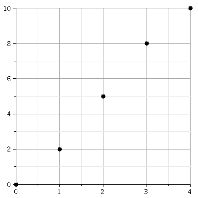
| > | # Plotting a set of points: Two different ways: |
| > | # Alternative 1 |
| > | pointplot([(0,0),(1,2),(2,5),(3,8),(4,10)], symbolsize=20,symbol=solidcircle,gridlines=true,view=[0..4,0..10]); |
|
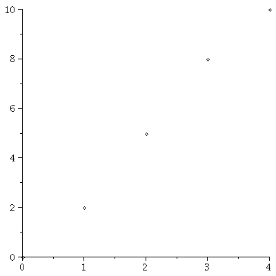
| > | # Alternative 2 |
| > |
| > | Xvalues:=[0,1,2,3,4]; # our x values |
| (1) |
| > | Yvalues:=[0,2,5,8,10]; # our y values |
| (2) |
| > | points:= {seq([Xvalues[n],Yvalues[n]],n=1..5)}:
|
| > | pointplot(points,view=[0..4,0..10]); |
 |
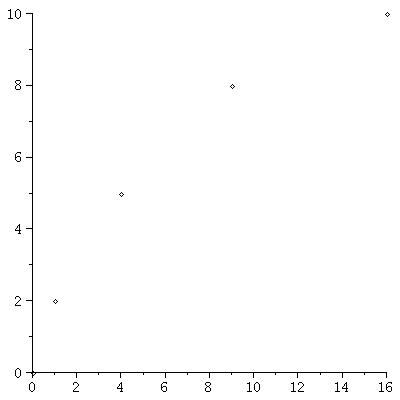
| > | # This second alternative is useful if we instead wanted to plot x_i^2 instead of x_i |
| > | pointsquare:= {seq([(Xvalues[n])^2,Yvalues[n]],n=1..5)}: |
| > | pointplot(pointsquare); |
 |
| > |
| > |
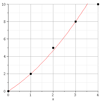
| > | # Putting two graphs on the same axis |
| > | p1:=pointplot([(0,0),(1,2),(2,5),(3,8),(4,10)], symbolsize=20,symbol=solidcircle,gridlines=true,view=[0..4,0..10]): |
| > | p2:=plot(2*x+0.5*x*(x-1)+(-1/6)*x*(x-1)(x-2),x=0..4): |
| > | display({p1,p2}); |
 |
| > |